Two families of orthogonal polynomials are named after Chebyshev because he explored their properties. These are prosaically named Chebyshev polynomials of the first and second kind.
I recently learned there are Chebyshev polynomials of the third and fourth kind as well. You might call these posthumous Chebyshev polynomials. They were not developed by Mr. Chebyshev, but they bear a family resemblance to the polynomials he did develop.
The four kinds of Chebyshev polynomials may be defined in order as follows.

It’s not obvious that these definitions even make sense, but in each case the right hand side can be expanded into a sum of powers of cos θ, i.e. a polynomial in cos θ. [1]
All four kinds of Chebyshev polynomials satisfy the same recurrence relation

for n ≥ 2 and P0 = 1 but with different values of P1, namely x, 2x, 2x − 1, and 2x + 1 respectively [2].
Plots
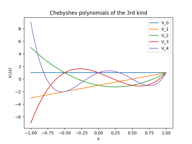
We can implement Chebyshev polynomials of the third kind using the recurrence relation above.
def V(n, x):
    if n == 0: return 1
    if n == 1: return 2*x - 1
    return 2*x*V(n-1, x) - V(n-2, x)
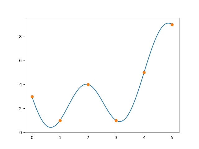
Here is a plot of Vn(x) for n = 0, 1, 2, 3, 4.
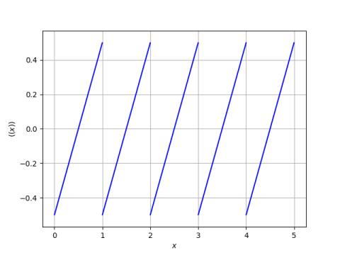
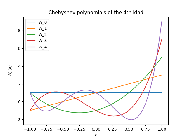
The code for implementing Chebyshev polynomials of the fourth kind is the same, except the middle line becomes
if n == 1: return 2*x + 1
Here is the corresponding plot.
Square roots
The Chebyshev polynomials of the first and third kind, and polynomials of the second and fourth kind, are related as follows:

To see that the expressions on the right hand side really are polynomials, note that Chebyshev polynomials of the first and second kinds are odd for odd orders and even for even orders [3]. This means that in the first equation, every term in T2n + 1 has a factor of √(1 + x) that is canceled out by the 1/√(1 + x) term up front. In the second equation, there are only even powers of the radical term so all the radicals go away.
You could take the pair of equations above as the definition of Chebyshev polynomials of the third and fourth kind, but the similarity between these polynomials and the original Chebyshev polynomials is more apparent in the definition above using sines and cosines.
The square roots hint at how these polynomials first came up in applications. According to [2], Chebyshev polynomials of the third and fourth kind
have been called “airfoil polynomials”, since they are appropriate for approximating the single square root singularities that occur at the sharp end of an airfoil.
Dirichlet kernel
There’s an interesting connection between Chebyshev polynomials of the fourth kind and Fourier series.
The right hand side of the definition of Wn is known in Fourier analysis as Dn, the Dirichlet kernel of order n.

The nth order Fourier series approximation of f, i.e. the sum of terms −n through n in the Fourier series for f is the convolution of f with Dn, times 2π.

Note that Dn(θ) is a function of θ, not of x. The equation Wn(cos θ) = Dn(θ) defines Wn(x) where x = cos θ. To put it another way, Dn(θ) is not a polynomial, but it can be expanded into a polynomial in cos θ.
Related posts
[1] Each function on the right hand side is an even function, which implies it’s at least plausible that each can be written as powers of cos θ. In fact you can apply multiple angle trig identities to work out the polynomials in cos θ.
[2] J.C. Mason and G.H. Elliott. Near-minimax complex approximation by four kinds of Chebyshev polynomial expansion. Journal of Computational and Applied Mathematics 46 (1993) 291–300
[3] This is not true of Chebyshev polynomials of the third and fourth kind. To see this note that V1(x) = 2x − 1, and W1(x) = 2x + 1, neither of which is an odd function.
![\left[ \begin{array}{cc|cc|cc|c} 0 & -1 & 0 & 0 & 0 & 0 & \cdots \\ 1 & 0 & 0 & 0 & 0 & 0 & \cdots \\ \hline 0 & 0 & 0 & -1 & 0 & 0 & \cdots \\ 0 & 0 & 1 & 0 & 0 & 0 & \cdots \\ \hline 0 & 0 & 0 & 0 & 0 & -1 & \cdots \\ 0 & 0 & 0 & 0 & 1 & 0 & \cdots \\ \hline \vdots & \vdots & \vdots & \vdots & \vdots & \vdots & \ddots \end{array} \right] \left[ \begin{array}{c} a_1 \\ b_1 \\ \hline a_2 \\ b_2 \\ \hline a_3 \\ b_3 \\ \hline \vdots \end{array} \right]](https://www.johndcook.com/hilbert_transform_matrix.svg)