The previous post mentioned Legendre polynomials. This post will give a brief introduction to these polynomials and a couple hints of how they are used in applications.
One way to define the Legendre polynomials is as follows.
- P0(x) = 1
- Pk are orthogonal on [−1, 1].
- Pk(1) = 1 for all k ≥ 0.
The middle bullet point means
![]()
if m ≠ n. The requirement that each Pk is orthogonal to each of its predecessors determines Pk up to a constant, and the condition Pk(1) = 1 determines this constant.
Here’s a plot of the first few Legendre polynomials.
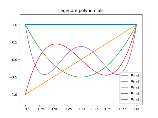
There’s an interesting pattern that appears in the white space of a graph like the one above when you plot a large number of Legendre polynomials. See this post.
The Legendre polynomial Pk(x) satisfies Legendre’s differential equation; that’s what motivated them.
![]()
This differential equation comes up in the context of spherical harmonics.
Next I’ll describe a geometric motivation for the Legendre polynomials. Suppose you have a triangle with one side of unit length and two longer sides of length r and y.
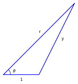
You can find y in terms of r by using the law of cosines:
![]()
But suppose you want to find 1/y in terms of a series in 1/r. (This may seem like an arbitrary problem, but it comes up in applications.) Then the Legendre polynomials give you the coefficients of the series.
![]()
Source: Keith Oldham et al. An Atlas of Functions. 2nd edition.
Should $\nu$ be $k$ in the differential equation?
That’s interesting. I knew I typed “k” and not “\nu”. I have a script that generates the HTML and the SVG, putting the LaTeX source into the HTML alt tag. And the alt text says “k.”
Turns out I had written about this before and had an older SVG file by the same name that used \nu.