Here’s an interesting theorem that leads to some aesthetically pleasing images. It’s known as the Japanese cyclic polygon theorem.
For all triangulations of a cyclic polygon, the sum of inradii of the triangles is constant. Conversely, if the sum of inradii is independent of the triangulation, then the polygon is cyclic.
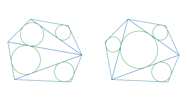
The image above shows two triangulations of an irregular hexagon. By the end of the post we’ll see the code that created these images, and we’ll see one more triangulations. And we’ll see that the sum of the radii of the circles is the same in each image.
Glossary
In case any of the terms in the theorem above are unfamiliar, here’s a quick glossary.
A triangulation of a polygon is a way to divide the polygon into triangles, with the restriction that the triangle vertices come from the polygon vertices.
A polygon is cyclic if there exists a circle that passes through all of its vertices. Incidentally, if a polygon has n + 2 sides, the number of possible triangulations is the nth Catalan number. More on that here.
The inradius of a triangle is the radius of the largest circle that fits inside the triangle. More on inner and outer radii here.
Equations for inradius and incenter
We’d like to illustrate the theorem by drawing some images and by adding up the inradii. This means we need to be able to find the inradius and the incenter.
The inradius of a triangle equals its area divided by its semiperimeter. The area we can find using Heron’s formula. The semiperimeter is half the perimeter.
The incenter is the weighted sum of the vertices, weighted by the lengths of the opposite sides, and normalized. If the vertices are A, B, and C, then the incenter is
![]()
where A is the vertex opposite side a, B is the vertex opposite side b, and C is the vertex opposite side c.
Python code
The following Python code will draw a triangle with its incircle. Calling this function for each triangle in the triangulation will create the illustrations we’re after.
from numpy import *
import matplotlib.pyplot as plt

def draw_triangle_with_incircle(A, B, C):
    a = linalg.norm(B - C)
    b = linalg.norm(A - C)
    c = linalg.norm(A - B)
    s = (a + b + c)/2
    r = sqrt(s*(s-a)*(s-b)*(s-c))/s
    center = (a*A + b*B + c*C)/(a + b + c)
    plt.plot([A[0], B[0]], [A[1], B[1]], color="C0")
    plt.plot([B[0], C[0]], [B[1], C[1]], color="C0")
    plt.plot([A[0], C[0]], [A[1], C[1]], color="C0")
    t = linspace(0, 2*pi)
    plt.plot(r*cos(t) + center[0], r*sin(t) + center[1], color="C2")
    return r
Next, we pick six points not quite evenly spaced around a circle.
angle = [0, 50, 110, 160, 220, 315] # degrees
p = [array([cos(deg2rad(angle[i])), sin(deg2rad(angle[i]))]) for i in range(6)]
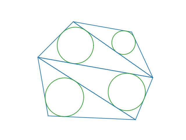
Now we draw three different triangulations of the hexagon defined by the points above. We also print the sum of the inradii to verify that each sum is the same.
def draw_polygon(triangles):
    rsum = 0
    for t in triangles:
        rsum += draw_triangle_with_incircle(p[t[0]], p[t[1]], p[t[2]])
    print(rsum)
    plt.axis("off")
    plt.gca().set_aspect("equal")
    plt.show()

draw_polygon([[0,1,2], [0,2,3], [0,3,4], [0,4,5]])
draw_polygon([[0,1,2], [2,3,4], [4,5,0], [0,2,4]])
draw_polygon([[0,1,2], [0,2,3], [0,3,5], [3,4,5]])
This produces the two images at the top of the post the one below. All the inradii sum are 1.1441361217691244 with a little variation in the last decimal place.
Fascinating, thank you for sharing this…