A logistic curve, sometimes called an S curve, looks different in different regions. Like the proverbial blind men feeling different parts of an elephant, people looking at different segments of the curve could come to very different impressions of the full picture.
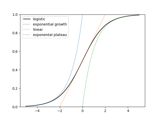
It’s naive to look at the left end and assume the curve will grow exponentially forever, even if the data are statistically indistinguishable from exponential growth.
A slightly less naive approach is to look at the left end, assume logistic growth, and try to infer the parameters of the logistic curve. In the image above, you may be able to forecast the asymptotic value if you have data up to time t = 2, but it would be hopeless to do so with only data up to time t = −2. (This post was motivated by seeing someone trying to extrapolate a logistic curve from just its left tail.)
Suppose you know with absolute certainty that your data have the form
![]()
where ε is some small amount of measurement error. The world is not obligated follow a simple mathematical model, or any mathematical model for that matter, but for this post we will assume that for some inexplicable reason you know the future follows a logistic curve; the only question is what the parameters are.
Furthermore, we only care about fitting the a parameter. That is, we only want to predict the asymptotic value of the curve. This is easier than trying to fit the b or c parameters.
Simulation experiment
I generated 16 random t values between −5 and −2, plugged them into the logistic function with parameters a = 1, b = 1, and c = 0, then added Gaussian noise with standard deviation 0.05.
My intention was to do this 1000 times and report the range of fitted values for a. However, the software I was using (scipy.optimize.curve_fit) failed to converge. Instead it returned the following error message.
RuntimeError: Optimal parameters not found: Number of calls to function has reached maxfev = 800.
When you see a message like that, your first response is probably to tweak the code so that it converges. Sometimes that’s the right thing to do, but often such numerical difficulties are trying to tell you that you’re solving the wrong problem.
When I generated points between −5 and 0, the curve_fit algorithm still failed to converge.
When I generated points between −5 and 2, the fitting algorithm converged. The range of a values was from 0.8254 to 1.6965.
When I generated points between −5 and 3, the range of a values was from 0.9039 to 1.1815.
Increasing the number of generated points did not change whether the curve fitting method converge, though it did result in a smaller range of fitted parameter values when it did converge.
I said we’re only interested in fitting the a parameter. I looked at the ranges of the other parameters as well, and as expected, they had a wider range of values.
So in summary, fitting a logistic curve with data only on the left side of the curve, to the left of the inflection point in the middle, may completely fail or give you results with wide error estimates. And it’s better to have a few points spread out through the domain of the function than to have a large number of points only on one end.
This brings back memories of the Tesla Model 3 production ramp-up some years ago.
I love your so-simple-they-can’t-ignore posts. Straight to the point.
This reminds me of a paper from the COVID-19 pandemic that claimed that exponential growth+uncertainty = exponential uncertainty. Therefore, the peak of the pandemic cannot be accurately forecasted. The logistic curve is “exponential inside”, so your analysis makes sense to me.
If you take weakly informative priors (e.g., normal(0, 5) on all the parameters with an and b constrained to be positive), then the posterior will at least be well defined. With 15 data points in (-5, -2), the uncertainty remains very wide. As you increase the number of data points, you will see the posterior interval narrow for the slope parameter (b) and concentrate around the true value. For example, with 10000 observations, the central 90% posterior interval is (0.91, 1.01) in the simulation I ran.
The intercept (c) and height (a) remain poorly identified even with 10K observations in the left tail where the curve is increasing exponentially. For instance you can adjust the height to compensate for the intercept and vice-versa. This weak identifiability will cause optimizers to fail as they can’t diagnose they have found the optimum value.
If you do pin both maximum value (a) and slope (b) to known values, then you can estimate the intercept (c) with only data from the left tail.
This model artifact goes away and everything is identifiable if you sample in a wider range.
Naively speaking, I think a “learning curve” would be an S-curve, wouldn’t it? Initial exposure (at least if one is engaged in the learning) can tap into enthusiasm. Then long, somewhat steady progress takes place through drudgery. Then there is the fine-tuning of expertise at the end. And curiously, this seems to hold sometimes on an aggregate level as well. A new subject becomes a hot topic, gradually shifts to slower but steady development, then picks up a few remaining results till it goes dormant.
Thoughts?