This post will give a detailed example of working in a field with nine elements. This is important because finite fields are not often treated concretely except for the case of prime order.
In my first post on Costas arrays I mentioned in a footnote that Lempel’s algorithm works more generally over any finite field, but I stuck to integers modulo primes to make things simpler.
In this post we’ll create a 7 × 7 Costas array by working in a field with 9 elements. Along the way we’ll explain in great detail how finite field arithmetic works, using the field with 9 elements as an example.
Prime powers are different
The order of a finite field can be any power of a prime. That is, a finite field can have q elements if (and only if) q = pk for some prime p and positive integer k.
If q is a prime, then any field with q elements is isomorphic to the integers mod q. Addition and multiplication are defined just as in the integers, except you always take the remainder by q after you add or multiply.
But if q is a prime power, things are different. So while multiplication in a field of 7 elements is simply multiplication mod 7, multiplication in a field of 9 elements is not multiplication mod 9.
Defining addition and multiplication
The field with nine elements can be defined as polynomials of the form ax + b where a and b are integers mod 3, i.e. a and b can take on the values 0, 1, or 2.
You can define addition in this little field the same way you always define polynomial addition, with the understanding that the coefficients are added mod 3. So, for example,
(2x + 1) + (x + 0) = 1
because the leading coefficient is 2 + 1, which reduces to 0 mod 3.
Multiplication is also defined as polynomial multiplication, with coefficient arithmetic being carried out mod 3, with one more step: after multiplying the polynomials, you divide by an irreducible quadratic polynomial and keep the remainder.
In general, if q = pk for some prime p and positive integer k, we define elements of our field to be polynomials of degree k − 1. When multiplying, we take the remainder after dividing by a fixed irreducible polynomial of degree k. In our example, k = 2, so we have first degree polynomials, and we take the remainder after dividing by a second degree polynomial.
Irreducible polynomials
The definition of multiplication brings up several questions.
- What is an irreducible polynomial?
- Can I always find one?
- How can I find one?
- Which one should I pick?
An irreducible polynomial is one that cannot be factored in the given context. Here we want a polynomial of degree 2, with coefficient in integers mod 3, that cannot be factored as the product of two linear polynomials with coefficients in integers mod 3.
There are plenty of irreducible polynomials. In our case, we have 36 to choose from. (This post explains a formula for counting how many irreducible polynomials there are of a given order over a given finite field.)
There are algorithms for finding irreducible polynomials, but this is beyond the scope of this post. Here’s one we will use:
x² + x + 2.
You could verify by brute force that this polynomial cannot be factored into
(ax + b)(cx + d)
where a and c are non-zero. There are 2 × 3 × 2 × 3 possibilities for a, b, c, and d, and you could verify that none of them work.
The difference choice makes
We said there are 36 irreducible polynomials we could choose. What about the other 35 we didn’t choose? They all lead to the same field, where by “same” we mean isomorphic. They generate different representations of the field, but there’s a direct correspondence (an isomorphism) between any two representations.
In one sense this is nothing to worry about, and in another sense it is. You’re not going to create something fundamentally different by choosing a different irreducible polynomial. If you and I pick different polynomials, we will agree on all the algebraic properties of our fields, but we could disagree on what the product of two particular polynomials is, like two people using two different units of measure. This can be an issue when doing finite field arithmetic with software: two software packages could give different results for a given product.
Primitive elements
An element g in a group G is primitive if every element of G is some power of g. For example, 3 is a primitive element of the integers mod 7 because if we take successive powers of 3 mod 7 we get
3, 2, 6, 4, 5, 1
and that’s all the non-zero elements of the integers mod 7. On the other hand, 2 is not a primitive element mod 7 because its powers are 2, 4, and 1. There’s no way to raise 2 to any power mod 8 and get 3, 5, or 6 out.
We need a primitive element of our finite field in order to carry out Lempel’s algorithm. It turns out we can use x as our primitive element. That is, every non-zero element of our field is a power of x. There are other primitive elements we could have chosen[1].
That statement may sound wrong. How, for example, can a power of x equal 2x + 1? We have to remember that we’re multiplying polynomials as described above, not as polynomials over real numbers.
When we multiply x by x, we get x² of course, but then we have to divide by our choice of irreducible polynomial, which we said above would be x² + x + 2.
If we divide x² by x² + x + 2 as we would in a high school algebra class, we get a quotient of 1 with a remainder of –x – 2. When we reduce the coefficients mod 3, we get 2x + 1. So in our world,
x² = 2x + 1.
OK, that takes some getting used to, but now what is x³? Well, it’s x times x² of course, but what is that? As before we’ll first pretend we’re doing high school algebra, then we’ll adjust. So x times 2x + 1 equals 2x² + x. When we divide by our irreducible polynomial, we get
2x² + x = 2(x² + x + 2) + 2x + 2
so the remainder is 2x + 2. Therefore in our context,
x³ = 2x + 2.
Powers of x
Lempel’s algorithm says to fill in the (i, j) square of our matrix if and only if
ai + aj = 1
where a is a generator of our field. In our case a is simply the polynomial x. Here i and j run from 1 through 7 (i.e. up to q – 2, and for us q = 9.)
We don’t need a full multiplication table; we only need powers of x. Here they are:
- x
- 2x + 1
- 2x + 2
- 2
- 2x
- x + 2
- x + 1
- 1
Incidentally, we could use this as a sort of table of logarithms. To multiply any two elements, scan the list to find out what power of x each element is. Then add the exponents, and see what element that corresponds to.
Filling in the Costas array
For each row i, we compute xi and then find which value of j satisfies
xj = 1 − xi.
So here we go.
When i = 1, 1 − xi = 1 − x = 2x + 1, and so j = 2.
When i = 2, 1 − xi = 1 − x² = 1 – (2x + 1) = x, and so j = 1.
When i = 3, 1 − xi = 1 − (2x+ 2) = x + 2, so j = 6.
When i = 4, 1 − xi = 1 − 2 = 2, so j = 4.
When i = 5, 1 − xi = 1 − 2x = x + 1, so j = 7.
We can figure out the rest by symmetry. As noted in the previous post, the pairs (i, j) are symmetric. So since (3, 6) is filled in, so is (6, 3). And since (5, 7) is filled in, so is (7, 5). We could have also figured out the case of i = 2 by symmetry.
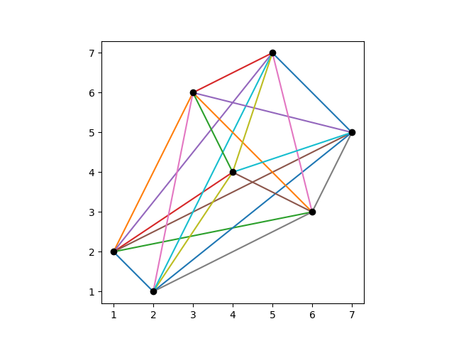
Visualizations
Here we visualize the Costas array we’ve found as in the earlier post. The line segments between filled in cells are all unique, so we draw cell positions and the connecting lines.
Here we translate all the lines to the origin to show that they’re distinct.
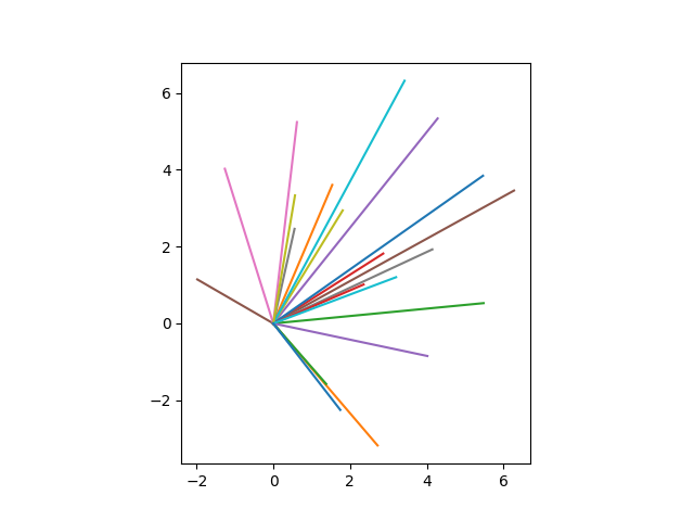
No two lines are the same, but some lines have the same slope with different lengths. To make it possible to see these, I added a small amount of randomness to the points before plotting them.
***
[1] The number of primitive polynomials of degree n in a field with q elements is φ(qn − 1)/n where φ is Euler’s totient function. In our example, n = 1 and q = 9, so there are φ(8) = 4 primitive polynomials to choose from. What are they?
Every non-zero element of our field is a power of x, so a primitive polynomial y must itself be a power of x, say y = xk. If yj = x, then we must have xjk = x. The multiplicative group of our field has 8 elements, so jk must be congruent to 1 mod 8. This means k must be 1, 3, 5, or 7. So our generators are x, x3 = 2x + 2 = x + 2, x5 = 2x, and x7 = x + 1.