A couple days ago I wrote about Costas arrays. In a nutshell, a Costas array of size n is a solution to the n rooks problem, with the added constraint that if you added wires between the rooks, no two wires would have the same length and slope. See the earlier post for more details.
The earlier post implemented the Lempel algorithm in Python. Here we’ll implement it in Mathematica. Lempel’s algorithm says to start with parameters p and a where p is a prime and a is a primitive root mod p [1]. Then you can create a Costas array of size n = p − 2 by filling in the (i, j) square if and only if
ai + aj = 1 mod p.
We can implement this in Mathematica by
    fill[i_, j_, p_, a_] := If[Mod[a^i + a^j, p] == 1, 1, 0]
    m[p_, a_] := Table[fill[i, j, p, a], {i, 1, p - 2}, {j, 1, p - 2}]
We could visualize the Costas array generated by p = 11 and a = 2 using ArrayPlot. The code
ArrayPlot[m[11, 2], Mesh -> All]
Generates the following image.
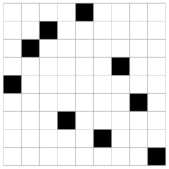
Note that the image is symmetric with respect to the main diagonal. That’s because our algorithm is symmetric in i and j. But Costas arrays are not always symmetrical, so this underscores the point that there is no known scalable algorithm for finding all Costas arrays.
In this example we started with knowing that 2 was a primitive root mod 11. We could have had Mathematica pick a primitive root mod p for us by calling PrimitiveRoot[p]
Just out of curiosity, let’s redo the example above, but instead of testing whether
ai + aj = 1 mod p.
we’ll just use ai + aj mod p.
The code
ArrayPlot[Table[Mod[2^i + 2^j, 11], {i, 1, 9}, {j, 1, 9}]]
produces the following image.

[1] Lempel’s algorithm generalizes to finite fields of any order, not just integers modulo a prime.