
I was digging into the Runge-Kutta method for solving differential equations and a line from [1] piqued my curiosity.
These calculations, which are not reproduced in Kutta’s paper (they are however in Huen (1900)), are very tedious.
The calculations are a set of eight constraints that the parameters of a fourth-order Runge-Kutta method must satisfy. I wondered how well Mathematica might have done at assisting Mr. Huen if it had been available in 1900.
I go into Runge-Kutta methods in this post. Here I’d like to concentrate on a step in the design of the methods, namely solving the set of equations alluded in the quote above.
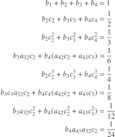
The first thing to note is that there are 10 variables and only 8 equations, and so the solution is not fully determined. What we think of as the fourth order Runge-Kutta method is in fact a fourth order Runge-Kutta method.
One could argue that we should have b2 = b3 and c2 = c3. With these additional equations, the system of equations has a unique solution, and Mathematic finds it easily.
eqs = {
    b1 + b2 + b3 + b4 == 1,
    b2*c2 + b3*c3 + b4*c4 == 1/2,
    b2*c2^2 + b3*c3^2 + b4*c4^2 == 1/3,
    b3*a32*c2 + b4*(a42*c2 + a43*c3) == 1/6,
    b2*c2^3 + b3*c3^3 + b4*c4^3 == 1/4,
    b3*c3*a32*c2 + b4*c4*(a42*c2 + a43*c3) == 1/8,
    b3*a32*c2^2 + b4*(a42*c2^2 + a43*c3^2) == 1/12,
    b4*a43*a32*c2 == 1/24,
    b2 == b3,
    c2 == c3
};

vars = {b1, b2, b3, b4, c2, c3, c4, a32, a42, a43};

solution = Solve[eqs, vars]
This returns the parameters used for the version of Runge-Kutta presented in every textbook.
If you keep the requirement b2 = b3 but substitute the requirement 2c2 = c3 for c‘s Mathematica will return the coefficients for the so-called Runge-Kutta 3/8 rule. This method has some slight advantages by some criteria.
In 1951 Gill [2] discovered a fourth order Runge-Kutta rule optimized for running in extremely constrained computer hardware. It’s a strange method, with irrational parameters, but one that was a very clever response to the limitations of its time.
[1] Hairer, Nørsett, and Wanner. Solving Ordinary Differential Equations I: Nonstiff Problems. Springer-Verlag 1987.
[2] A. Gill. A process for the step-by-step integration of differential equations in an automatic digital computing machine. Proc. Cambridge Philos. Soc., vol 27, pp 95–108.