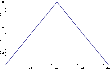
Suppose you have uniform random samples from the interval [0, 1]. If you add a large number of such samples together, the sum has an approximately normal distribution according to the central limit theorem. But how many do you have to add together to get a good approximation to a normal? Well, two is clearly not enough. Here’s what the density looks like for the sum of two uniform values.

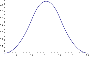
But look what happens when we add three uniforms together. If you’re very familiar with the normal distribution and have a good eye, you might be able to tell that the density is a little flat at the top.

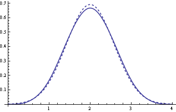
Here’s a graph that shows the distribution for a sum of four uniforms. The dotted curve is the graph of the normal distribution with the same mean and variance as the sum of the four uniforms. If the two graphs were not on top of each other, hardly anyone could tell which was the normal and which was the sum of uniforms.

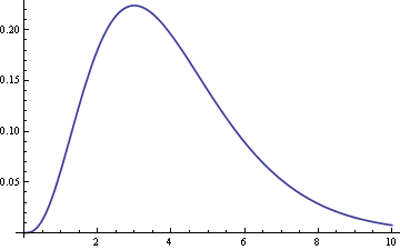
Note that this fast convergence to a normal distribution is a special property of uniform random variables. The sum of four exponential random variables, for example, does not look nearly so normal.

Here’s the analytic expression for the density of the sum of n uniform random variables that was used to produce these graphs.
Here the notation z+ stands for the positive part of z, i.e. the expression z+ equals z if z is positive and equals 0 otherwise.
According to Feller’s classic book, the density result above was discovered by Lagrange. Feller gives a series of exercises leading up to this result. First he gives the distribution function for the sum of n-sided dice and asks the reader to prove the result. Then the reader is asked to take the limit as the number of sides on each dice goes to infinity to derive the result for uniform random variables.
John Venier left a comment to a previous post about the following method for generating a standard normal: add 12 uniform random variables and subtract 6. Note that this is not just any normal distribution but a standard normal, i.e. mean 0 and variance 1. Since the variance of a single uniform random variable is 1/12, adding 12 such values makes the variance 1. How good is the generator he describes? The maximum difference between the CDF of his generator and the CDF of a standard normal is about 0.00234.
Related post: Rolling dice for normal samples

Thanks for doing the math, John. I was curious how good it was. Sounds plenty good. I think we (and I intentionally include myself) sometimes worry too much about the quality of PRNGs and approximations. Fortunately these days it is not usually not much harder to make the best choice than it is to make a bad one; the real trick is knowing when your choice is bad and that there is a better alternative. But if it looks like a Herculean task to get a slightly better PRNG we may do well to recall what was used (very successfully) in the Manhattan project. But I digress.
In fact, I wrote a long comment and redacted almost all of it due to a bad case of digression to the mean. The key consideration is the symmetry of the underlying distribution. A few practical experiments are enlightening, and may well change your attitude about a lot of statistics. There are many similar places in statistics where the practical seems at odds with the theory and especially the classical presentation of statistics. I think this is a fascinating topic in its own right and have examined it quite a bit, but it is out of place here.
It’s interesting to compare numerical error and programming error. Generating 12 uniform values is probably a few times more expensive than something like Marsaglia’s ziggurat algorithm. On the other hand, the uniform average method is so simple, it’s hard to imagine programming it incorrectly. A bug could more easily hide in code for Marsaglia’s algorithm.
John,
just a couple of notes: Feller’s classic for free is available on scribd.com I am not sure how it is possible that this and other good books are there, but they have been there for quite a while.
Second, it’s interesting how all modern probability books (Durrett, Pollard, Kallenberg, even Billingsley) do not have such beautifully worked-out numerical examples.
What about the margins John?
The normal distribution still has value outside of -6 to 6, the sum of 12 uniform random variables does not.
Considering that anything beyond a 6 standard deviation span of the normal is generally accepted to be insignificant, it probably does not matter.
In Feller’s book the expression has n! instead of (n-1)! and (x-k)^n instead of (x-k)^(n-1)
Would you please explain why is this difference?
Tanvir, we may be talking about PDF versus CDF. In my blog post, I gave the PDF. Feller (page 285 of the third edition, problem 20) gives the CDF.
Hi John,
Could you provide a simple code e.g., Python code, to implement the given formula? I will understand much easier the concept then.
I had also difficulty in very first part while the rest was understandable!
“Suppose you have uniform random samples from the interval [0, 1].”
>>> s = scipy.rand(k,n)
“If you add a large number (k) of such samples together, the sum …”(????)
>>> s1 = s.flatten() #all samples to one big sample
or
>>> s1 = scipy.sum(s) #k sums
however none of the results above have normal distribution!
Thanks.
Developer
Personally, considering how very “non-normal” the uniform distribution is, I am always amazed how close to a normal we get summing just two uniforms (CLT requires n->infinity and n=2 is a long, long way from that)!
I believe the sum (or possibly average) of n uniforms is sometimes called Bartlett’s distribution but I have no reference for the origin of this name (likely because it follows Stigler’s law).
A gloss on this blog, focusing on the qualitative nature of the PDFs of sums of iid uniform variables, appears in a StackExchange thread at http://stats.stackexchange.com/questions/41467.
It’s called the Irwin-Hall distribution.
Should there not be a 2 in the denominator? Why the difference from the wiki entry?