Suppose you did a pilot study with 10 subjects and found a treatment was effective in 7 out of the 10 subjects.
With no more information than this, what would you estimate the probability to be that the treatment is effective in the next subject? Easy: 0.7.
Now what would you estimate the probability to be that the treatment is effective in the next two subjects? You might say 0.49, and that would be correct if we knew that the probability of response is 0.7. But there’s uncertainty in our estimate. We don’t know that the response rate is 70%, only that we saw a 70% response rate in our small sample.
If the probability of success is p, then the probability of s successes and f failures in the next s + f subjects is given by

But if our probability of success has some uncertainty and we assume it has a beta(a, b) distribution, then the predictive probability of s successes and f failures is given by

where

In our example, after seeing 7 successes out of 10 subjects, we estimate the probability of success by a beta(7, 3) distribution. Then this says the predictive probability of two successes is approximately 0.51, a little higher than the naive estimate of 0.49. Why is this?
We’re not assuming the probability of success is 0.7, only that the mean of our estimate of the probability is 0.7. The actual probability might be higher or lower. The predictive probability calculates the probability of outcomes under all possible values of the probability, then creates a weighted average, weighing each probability of success by the probability of that value. The differences corresponding to probability above and below 0.7 approximately balance out, but the former carry a little more weight and so we get roughly what we did before.
If this doesn’t seem right, note that mean and median aren’t the same thing for asymmetric distributions. A beta(7,3) distribution has mean 0.7, but it has a probability of 0.537 of being larger than 0.7.
If our initial experiment has shown 70 successes out of 100 instead of 7 out of 10, the predictive probability of two successes would have been 0.492, closer to the value based on point estimate, but still different.
The further we look ahead, the more difference there is between using a point estimate and using a distribution that incorporates our uncertainty. Here are the probabilities for the number of successes out of the next 100 outcomes, using the point estimate 0.3 and using predictive probability with a beta(7,3) distribution.
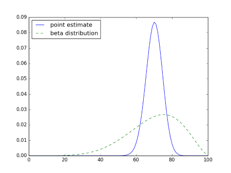
So if we’re sure that the probability of success is 0.7, we’re pretty confident that out of 100 trials we’ll see between 60 and 80 successes. But if we model our uncertainty in the probability of response, we get quite a bit of uncertainty when we look ahead to the next 100 subjects. Now we can say that the number of responses is likely to be between 30 and 100.
The second image has a broken link.
Must be a cache problem. I see the image in my browser. I’ll try to fix it.
John Cochrane made a similar point about the distribution of cumulative risky financial returns a few years ago:
http://johnhcochrane.blogspot.com/2013/07/the-value-of-public-sector-pensions.html
This is how some public pension funds got into trouble, by assuming point estimations for returns on risky investments, like 8% per year.
I’m also seeing broken images.
Easy: 0.7? I thought that probability would be (7+1)/(10+2)=2/3 as per https://en.wikipedia.org/wiki/Rule_of_succession
If so, then p(treatment is effective in the next two subjects) = (7+1)/(10+2) x (8+1)/(11+2) = 6/13 = 0.461538
Thoughts? Comments?
Can you recommend good book on this topic? (how to use beta distribution for prediction)
Josh: Any book on Bayesian statistics that covers predictive probability will probably use a beta distribution as its first example since that’s the easiest case. See, for example, Bayesian Data Analysis by Gelman et al.
Also broken images. Have only loaded the page once. Tried in both Chrome & Safari.
The broken images are fixed now :-)