This post serves two purposes. It will empirically explore a question in number theory and demonstrate quantile-quantile (q-q) plots. It will shed light on a question raised in the previous post. And if you’re not familiar with q-q plots, it will serve as an introduction to such plots.
The previous post said that for almost all x > 1, the fractional parts of the powers of x are uniformly distributed. Although this is true for almost all x, it can be hard to establish for any particular x. The previous post ended with the question of whether the fractional parts of the powers of 3/2 are uniformly distributed.
First, lets just plot the sequence (3/2)n mod 1.
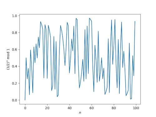
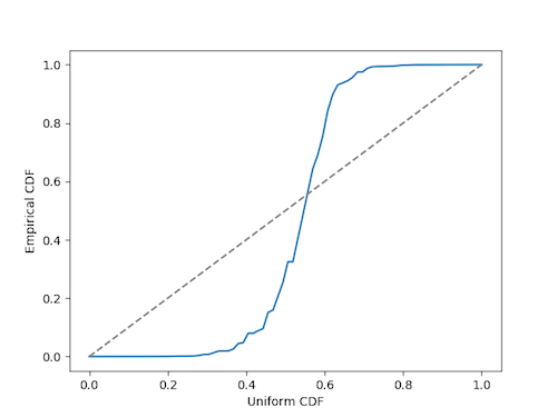
Looks kinda random. But is it uniformly distributed? One way to tell would be to look at the empirical cumulative distribution function (ECDF) and see how it compares to a uniform cumulative distribution function. This is what a quantile-quantile plot does. In our case we’re looking to see whether something has a uniform distribution, but you could use a q-q plot for any distribution. It may be most often used to test normality by looking at whether the ECDF looks like a normal CDF.
If a sequence is uniformly distributed, we would expect 10% of the values to be less than 0.1. We would expect 20% of the values to be less than 0.2. Etc. In other words, we’d expect the quantiles to line up with their theoretical values, hence the name “quantile-quantile” plot. On the horizontal axis we plot uniform values between 0 and 1. On the vertical axis we plot the sorted values of (3/2)n mod 1.
A qq-plot indicates a good fit when values line up near the diagonal, as they do here.
For contrast, let’s look at a qq-plot for the powers of the plastic constant mod 1.
Here we get something very far from the diagonal line. The plot is flat on the left because many of the values are near 0, and it’s flat on the right because many values are near 1.
Incidentally, the Kolmogorov-Smirnov goodness of fit test is basically an attempt to quantify the impression you get from looking at a q-q plot. It’s based on a statistic that measures how far apart the empirical CDF and theoretical CDF are.
Does this depend on the base?
In binary, 3/2 = 1.1, so that (3/2)^n will have a 1 in the nth position of the mantissa for all n, and that will be the last nonzero entry in that mantissa. That certainly _seems_ like it wouldn’t result in a uniform distribution of mantissas — but the set of mantissas whose last ‘1’ happens ‘early’ have measure zero, so maybe it does converge in probability…