Exponential sums are a specialized area of math that studies series with terms that are complex exponentials. Estimating such sums is delicate work. General estimation techniques are ham-fisted compared to what is possible with techniques specialized for these particular sums. Exponential sums are closely related to Fourier analysis and number theory.
Exponential sums also make pretty pictures. If you make a scatter plot of the sequence of partial sums you can get surprising shapes. This is related to the trickiness of estimating such sums: the partial sums don’t simply monotonically converge to a limit.
The exponential sum page at UNSW [link went away] suggests playing around with polynomials with dates in the denominator. If we take that suggestion with today’s date, we get the curve below:
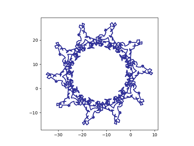
These are the partial sums of exp(2πi f(n)) where f(n) = n/10 + n²/7 + n³/17.
[Update: You can get an image each day for the current day’s date here.]
Here’s the code that produced the image.
    import matplotlib.pyplot as plt
    from numpy import array, pi, exp, log

    N = 12000
    def f(n):
        return n/10 + n**2/7 + n**3/17

    z = array( [exp( 2*pi*1j*f(n) ) for n in range(3, N+3)] )
    z = z.cumsum()

    plt.plot(z.real, z.imag, color='#333399')
    plt.axes().set_aspect(1)
    plt.show()
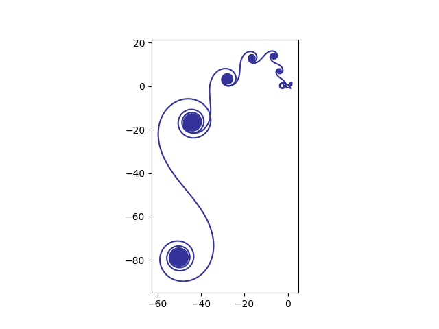
If we use logarithms, we get interesting spirals. Here f(n) = log(n)4.1.
And we can mix polynomials with logarithms. Here f(n) = log(n) + n²/100.
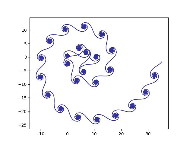
In this last image, I reduced the number of points from 12,000 to 1200. With a large number of points the spiral nature dominates and you don’t see the swirls along the spiral as clearly.
I Made An exp Sum with the birthday of my first grandchild yesterday. (8 oct 2017). I put the Pic on a Card with the text : a suiting crown for Céline on her birthday.
In that first example, the shapes remind me of Brusqueness figures. We a bit of work, I bet you could actually fit to a given silhouette.
^^^ oops. Serious autocorrect fail!
… Rubinesque figures. With a bit …
John,
In your sample code, what is 1j ?
The summation at UNSW is e^(2*pi*i*f(n))
Thanks,
Chuck
reducing the expression e^(2 * pi * i * f(n), I note that e^(pi * i) = -1
so I reduce the expression to (-1)^(2 * f(n))
2*f(n) = ( (n/mm) + (n^2/dd) + (n^3/yy)) yields a fraction
thus, I have eliminated the i
correct?
regards,
Chuck
1j is the imaginary unit in Python, i.e. “i” in math notation.
thanks John!
-Chuck
@Chuck
The rule (e^x)^y=e^(xy) holds if both x and y are real, but doesn’t always hold for complex values.
Here’s the code in Mathematica (it runs a bit slow)
m = 2000;
day = 21;
month = 11;
year = 17;
f[n_] = n/day + n^2/month + n^3/year;
g[x_] = Exp[2*Pi*I*f[x]];
z = Array[g, m + 1, {3, m + 3}];
z = Accumulate[z];
p = ListPlot[{Re[#], Im[#]} & /@ z, PlotRange -> Automatic,
ImagePadding -> 40, AspectRatio -> 1,
FrameLabel -> {{Im, None}, {Re, “complex plane”}},
PlotStyle -> Directive[Red, PointSize[.02]], Joined -> True];
Show[p]
what version of python and matplotlib was the python code run under?
regards,
-chuck rothauser
ok, I just answered my own question – the python code works fine under version 3.6 of python – I have a fedora workstation that has versions 2.7 and 3.6 and yup 2.6 was the default LOL
-chuck rothauser
I took the code John posted and added date input function with error checking :-)
-Chuck
import matplotlib.pyplot as plt, time
from numpy import array, pi, exp, log, e
valid = False
while not valid:
date_str = input(“Enter Date(mm/dd/yy):”)
try:
time.strptime(date_str, “%m/%d/%y”)
valid = True
except ValueError:
print(“Invalid Format For Date”)
valid = False
print(date_str)
m = int(date_str[0:2])
d = int(date_str[3:5])
y = int(date_str[6:8])
N = 12000
def f(n):
return n/m + n**2/d + n**3/y
z = array( [exp( 2*pi*1j*f(n) ) for n in range(3, N+3)] )
z = z.cumsum()
plt.plot(z.real, z.imag, color=’#333399′)
plt.axes().set_aspect(1)
plt.show()
looks like 2018 will produce less interesting patterns compared to 2017.. 2017 is prime and 2018 is not!!
correct me if i am wrong
2018 will produce simpler images since lcm(m, d, 18) is typically smaller than lcm(m, d, 17). The images are particularly simple now that m = 1, but some more complex images are coming.