I’ve playing around with driven Van der Pol oscillators.
![]()
The cosine term is the driving function. You can see a variety of behavior depending on the interaction between the driving frequency and the natural frequency, along with the other parameters. Sometimes you get periodic solutions and sometimes you get chaotic behavior.
Here’s the Python code I started with
    a, b = 0, 300
    t = linspace(a, b, 1000)
    mu = 9
    T = 10

    def vdp_driven(t, z):
        x, y = z
        return [y, mu*(1 - x**2)*y - x + cos(2*pi*t/T)]

    sol = solve_ivp(vdp_driven, [a, b], [1, 0], t_eval=t)
    plt.plot(sol.y[0], sol.y[1])
The first phase plot looked like this:
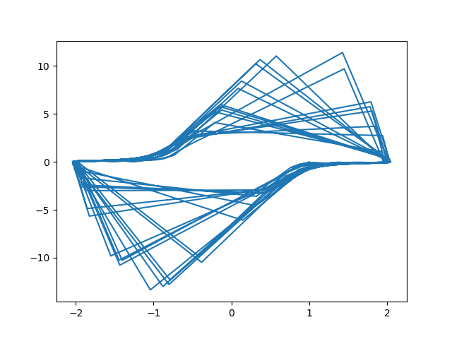
That’s weird. So I increased the number of solution points by changing the last argument to linspace from 1,000 to 10,000. Here’s the revised plot.
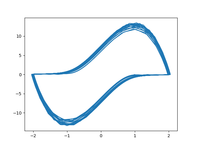
That’s a lot different. What’s going on? The solutions to the driven Van der Pol equation, and especially their derivative, change abruptly, so abruptly that if there’s not an integration point in the transition zone you get the long straight lines you see above. With more resolution these lines go away. This is understandable when you look at the plot of the solution:
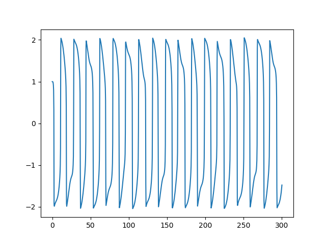
and of its derivative:
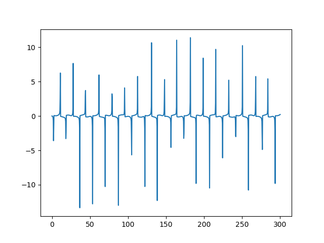
The solution looks fairly regular but the varying amplitudes of the derivative highlight the irregular behavior. The correct phase plot is not as crazy as the low-resolution version suggests, but we can see that the solution does not quickly settle into a limit cycle as it does in the undriven case.