There is no precise definition of what it means for a differential equation to be stiff, but essentially it means that implicit methods will work much better than explicit methods. The first use of the term [1] defined stiff equations as
equations where certain implicit methods, in particular BDF, perform better, usually tremendously better, than explicit ones.
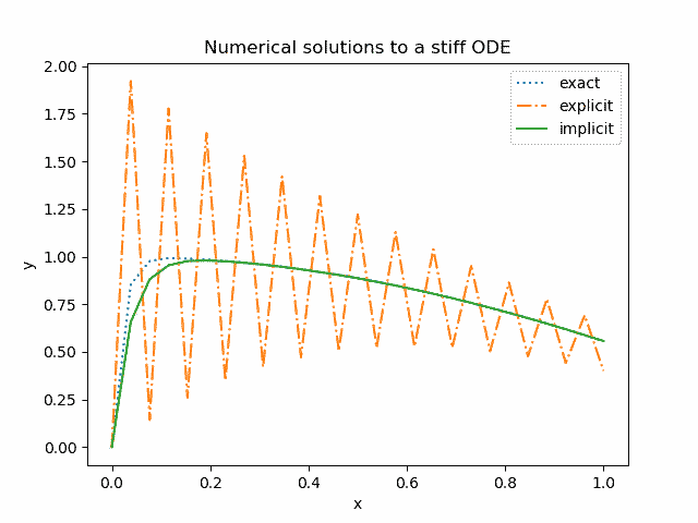
We’ll explain what it means for a method to be explicit or implicit and what BDF means. And we’ll give an example where the simplest implicit method performs much better than the simplest explicit method. Here’s a plot for a little foreshadowing.
Euler’s method
Suppose you have a first order differential equation
![]()
with initial condition y(0) = c. The simplest numerical method for solving differential equations is Euler’s method. The idea is replace the derivative y‘ with a finite difference
![]()
and solve for y(x + h). You start out knowing y(0), then you solve for y(h), then start over and use y(h) to solve for y(2h), etc.
Explicit Euler method
There are two versions of Euler’s method. The explicit Euler method uses a forward difference to approximate the derivative and the implicit Euler method uses a backward difference.
Forward difference means that at a given point x, we approximate the derivative by moving ahead a step h
![]()
and evaluating the right hand side of the differential equation at the current values of x and y, i.e.
![]()
and so
![]()
Implicit Euler method
The idea of the implicit Euler method is to approximate the derivative with a backward difference
![]()
which leads to
![]()
or equivalently
![]()
The text quoted at the top of the post referred to BDF. That stands for backward difference formula and we have an example of that here. More generally the solution at a given point could depend on the solutions more than one time step back [2].
This is called an implicit method because the solution at the next time step,
![]()
appears on both sides of the equation. That is, we’re not given the solution value explicitly but rather we have to solve for it. This could be complicated depending on the nature of the function f. In the example below it will be simple.
Example with Python
We’ll take as our example the differential equation
![]()
with initial condition y(0) = 0.
The exact solution, written in Python, is
    def soln(x):
        return (50/2501)*(sin(x) + 50*cos(x)) - (2500/2501)*exp(-50*x)
Here’s the plot again from the beginning of the post. Note that except at the very beginning, the difference between the implicit method approximation and exact solution is too small to see.
In the plot above, we divided the interval [0, 1] into 27 steps.
x = linspace(0, 1, 27)
and implemented the explicit and implicit Euler methods as follows.
    def euler_explicit(x):
        y = zeros_like(x)
        h = x[1] - x[0]
        for i in range(1, len(x)):
            y[i] = y[i-1] -50*h*(y[i-1] - cos(x[i]))
        return y

    def euler_implicit(x):
        y = zeros_like(x)
        h = x[1] - x[0]
        for i in range(1, len(x)):
            y[i] = (y[i-1] + 50*h*cos(x[i])) / (50*h + 1)
        return y
Here’s a plot of the absolute error in both solution methods. The error for the implicit method, too small to see in the plot, is on the order of 0.001.
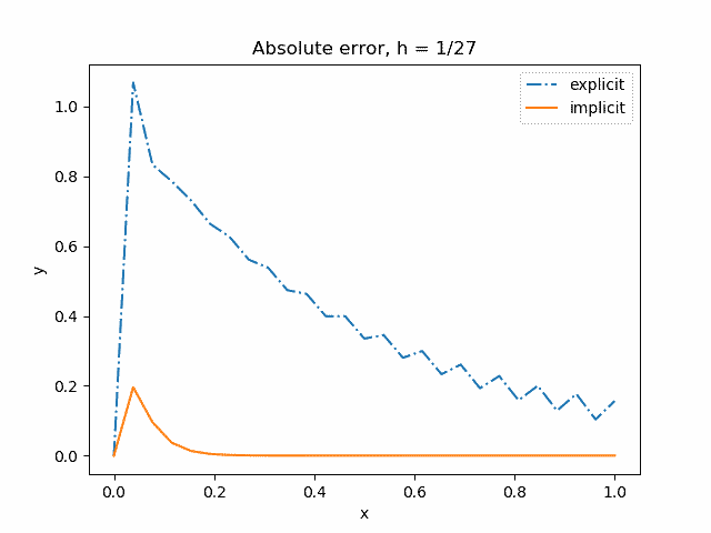
In the plots above, we use a step size h = 1/27. With a step size h = 1/26 the oscillations in the explicit method solution do not decay.
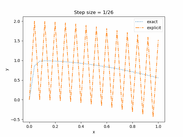
And with a step size h = 1/25 the oscillations grow.
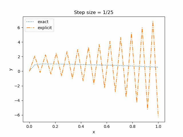
The explicit method can work well enough if we take the step size smaller, say h = 1/50. But smaller step sizes mean more work, and in some context it is not practical to use a step size so small that an explicit method will work adequately on a stiff ODE. And if we do take h = 1/50 for both methods, the error is about 10x larger for the explicit method.
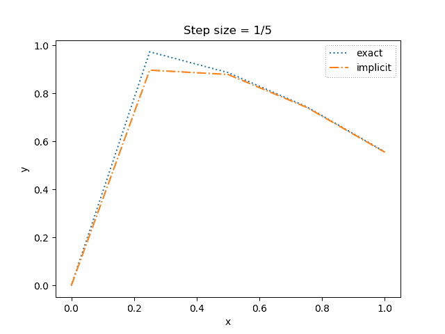
By contrast, the implicit method does fairly well even with h as large as 1/5.
(The “exact” solution here means the analytical solution sampled at six points just as the numerical solution is available at six points. The actual solution is smooth; the sharp corner comes from sampling the function at too few points for it to look smooth.)
Related posts
[1] C. F. Curtiss and J. O. Hirschfelder (1952). Integration of stiff equations. Proceedings of the National Academy of Sciences. Vol 38, pp. 235–243.
[2] This may be confusing because we’re still evaluating y at x + h, and so you might think there’s nothing “backward” about it. The key is that we are approximating the derivative of y at points that are backward relative to where we are evaluating f(x, y). On the right side, we are evaluating y at an earlier point than we are evaluating f(x, y).
I believe the second and third equations are missing a “y” in the numerator.
Quote: “The implicit method can work well if we take the step size smaller, say h = 50.”
Probably, you want to write “h = 1/50”.
“The implicit method can work well if we take the step size smaller” -> implicit should be explicit
It seems that in the implicit method equation, one should replace y+h with
y(x+h)
The implicit Euler method looks a bit like a first-order step towards a 3rd or 4th order Runga Kutta integration.