Leapfrog integrator

The so-called “leapfrog” integrator is a numerical method for solving differential equations of the form

where x is a function of t. Typically x is position and t is time.

This form of equation is common for differential equations coming from mechanical systems. The form is more general than it may seem at first. It does not allow terms involving first-order derivatives, but these terms can often be eliminated via a change of variables. See this post for a way to eliminate first order terms from a linear ODE.

The leapfrog integrator is also known as the Störmer-Verlet method, or the Newton-Störmer-Verlet method, or the Newton-Störmer-Verlet-leapfrog method, or …

The leapfrog integrator has some advantages over, say, Runge-Kutta methods, because it is specialized for a particular (but important) class of equations. For one thing, it solves the second order ODE directly. Typically ODE solvers work on (systems of) first order equations: to solve a second order equation you turn it into a system of first order equations by introducing the first derivative of the solution as a new variable.

For another thing, it is reversible: if you advance the solution of an ODE from its initial condition to some future point, make that point your new initial condition, and reverse time, you can step back to exactly where you started, aside from any loss of accuracy due to floating point; in exact arithmetic, you’d return to exactly where you started.

Another advantage of the leapfrog integrator is that it approximately conserves energy. The leapfrog integrator could perform better over time compared to a method that is initially more accurate.

Here is the leapfrog method in a nutshell with step size h.

$\begin{align*} x_{i+1} &= x_i + v_i h + \frac{1}{2} f(x_i) h^2 \\ v_{i+i} &= v_i + \frac{1}{2}\left(f(x_i) + f(x_{i+1})\right) h \end{align*}$

And here’s a simple Python demo.

    import numpy as np
    import matplotlib.pyplot as plt
    
    # Solve x" = f(x) using leapfrog integrator
    
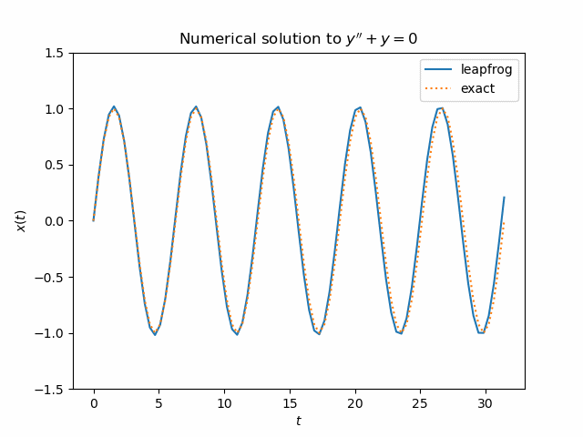
    # For this demo, x'' + x = 0
    # Exact solution is x(t) = sin(t)
    def f(x):
        return -x
    
    k = 5               # number of periods
    N = 16              # number of time steps per period
    h = 2*np.pi/N       # step size
    
    x = np.empty(k*N+1) # positions
    v = np.empty(k*N+1) # velocities
    
    # Initial conditions
    x[0] = 0
    v[0] = 1
    anew = f(x[0])
    
    # leapfrog method
    for i in range(1, k*N+1):
        aold = anew
        x[i] = x[i-1] + v[i-1]*h + 0.5*aold*h**2
        anew = f(x[i])
        v[i] = v[i-1] + 0.5*(aold + anew)*h

Here’s a plot of the solution over five periods.

There’s a lot more I hope to say about the leapfrog integrator and related methods in future posts.

One thought on “Leapfrog integrator”

Jakub Narębski

14 July 2020 at 02:30

There are various variants of Verlet / leapfrog integrator. The one I have encountered most often looks like the following, which looks like Euler integrator on first glance (the equation in the post is velocity Verlet variant)…

v_{i+1/2} = v_{i-1/2} + f(x_{i})*h
x_{i+1} = x_{i} + v_{i+1/2}*h

The above form has the disadvantage in that it needs some other method to start (or otherwise needs help starting the iteration), unless one does not care that it solves the problem with different starting conditions.

I have also stumbled upon a warning that classic Verlet method does not work well with adaptive integration step ‘h’.

I have encountered mentions of Yoshida integrator and Hermite–Obreschkoff method.

Comments are closed.

More on ODE solvers

One thought on “Leapfrog integrator”