Ancient estimate of π and modern numerical analysis

Posted on 30 July 2023 by John

A very crude way to estimate π would be to find the perimeter of squares inside and outside a unit circle.

Circle with inscribed and circumscribed squares

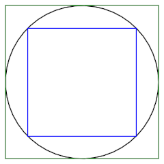
The outside square has sides of length 2, so 2π < 8. The inside square has sides of length 2/√2, so 8/√2 < 2π. This tells us π is between 2.82 and 4. Not exciting, but it’s a start.

Finding the perimeter of an inscribed hexagon and a circumscribed hexagon would be better. Finding the perimeter of inscribed and circumscribed n-gons for larger values of n would be even better.

Archimedes and successors

Archimedes (287–212 BC) estimated π using inscribed and circumscribed 96-gons.

Aryabhata (476–450 AD) used Archimedes idea with n = 384 (3 × 2⁷) and Vièta (1540–1603) used n = 39,3216 (3 × 2¹⁷).

Accuracy

The perimeter of a regular n-gon inscribed in the unit circle is

T_n = 2n sin(π/n)

and the perimeter of a regular n-gon circumscribed on the unit circle is

U_n = 2n tan(π/n).

We look at these formulas and see a way to calculate T_n and U_n by plugging π/n into functions that calculate sine and cosine. But Archimedes et al had geometric ways of computing T_n and U_n and used these to estimate π.

We can use the formulas above to evaluate the bounds above.

Archimedes: 3.1410 < π < 3.1427.

Aryabhata: 3.14155 < π < 3.14166.

Vièta: 3.14159265355 < π < 3.1415926536566.

Extrapolation

In 1654, Huygens discovered that algebraic combinations of the perimeter estimates for an n-gon and an (n/2)-gon could be better than either. So, for example, while Archimedes estimate based on a 96-gon is better than an estimate based on a 48-gon, you could combine the two to do better than both.

His series were

S_n = (4T_n − T_n/2)/3

and

V_n = (2U_n + T_n/2)/3

Huygens did not prove that S_n and V_n were lower and upper bounds on 2π, but they are, and are much better than T_n and U_n. Using a 48-gon and a 96-gon, for example, Huygens could get twice as many correct digits as Archimedes did with a 96-gon alone.

From a modern perspective, Huygens’ expressions can be seen as a first step toward what Richardson called “the deferred approach to the limit” in 1927, or what is often called Richardson extrapolation. By expanding the expressions for T_n and U_n as Taylor series in h = 1/n, we can take algebraic combinations of expressions for varying values of h that eliminate small powers of h, increasing the order of the approximation.

Huygens came up with expressions that canceled out terms of order h² and leaving terms of order h⁴. (The odd-order terms were already missing from sin(h)/h and tan(h)/h.)

Milne (1896–1950) came up with a systematic approach that could, for example, use polygons with n, n/2, and n/4 sides to come up with an approximation for π with order h⁶ and to form approximation with order equal to any even power of h. By making clever use of perimeter values known to Archimedes, Milne could obtain more accurate results than those that Aryabhata and Vièta obtained.

Richardson saw a general pattern in the work of Milne and others. We take expressions involving limits as h goes to 0, i.e. derivatives, and to do some manipulation before letting some h go to 0. Taking the derivative would be to take a limit immediately. But if we let some terms cancel each other out before taking the limit, we can get approximations that converge more quickly.

Richardson developed this idea used it as a way to solve a variety of problems more efficiently, such as numerical integration and numerically solving differential equations.

References

[1] L. F. Richardson. The deferred approach to the limit. I. Single lattice, Philos. Trans. Roy. Soc. London Ser. A, 226, pp. 299-349 (1927)

[2] D. C. Joyce. Survey of Extrapolation Process in Numerical Analysis by SIAM Review , Oct., 1971, Vol. 13, No. 4, pp. 435–490

Halley’s variation on Newton’s method

Posted on 4 July 2023 by John

Newton’s method for solving f(x) = 0 converges quickly once it starts to converge. Specifically, it converges quadratically: the error is roughly squared at each step. This means that the number of correct decimal places doubles at each iteration of Newton’s method.

Doubling the number of decimal places is nice, but what if we could triple the number of correct decimals at each step? Edmond Halley, best known for the comet that bears his name, came up with a way to do just that. Newton’s method converges quadratically, but Halley’s method converges cubically.

Newton’s method updates iterations using the rule

$x_{n+1} = x_n + \frac{f(x_n)}{f'(x_n)}$

Halley’s variation uses the rule

$x_{n+1} = x_n - \frac{1}{\dfrac{f'(x_n)}{f(x_n)} - \dfrac{f''(x)}{2f'(x)}}$

Halley’s method makes more progress per iteration, but it also takes more work per iteration, and so in practice it’s not usually an improvement over Newton’s method. But in some cases it could be.

Evaluating efficiency

In root-finding problems, the function f is usually relatively time-consuming to evaluate. We can assume nearly all the work in root-finding goes into evaluating f and its derivatives, and we can ignore the rest of the arithmetic in the method.

Newton’s method requires evaluating the function f and its derivative f ′. Halley’s method requires these function evaluates as well and also requires evaluating the second derivative f ′′.

Three iterations of Newton’s method make as much progress toward finding a root as two iterations of Halley’s method. But since Newton’s method requires two function evaluations and Halley’s method requires three, both require six function evaluations to make the same amount of progress. So in general Halley’s method is not an improvement over Newton’s method.

When Halley might be better

Suppose we had a way to quickly compute the second derivative of f at a point from the values of f and its first derivative at that point, rather than by having to evaluate the second derivative explicitly. In that case two iterations of Halley’s method might make as much progress as three iterations of Newton’s method but with less effort, four function evaluations rather than six.

Many of the functions that are used most in applied mathematics satisfy 2nd order differential equations, and so it is common to be able to compute the second derivative from the function and its derivative.

For example, suppose we want to find the zeros of Bessel functions J_ν. Bessel functions satisfy Bessel’s differential equation; that’s where Bessel functions get their name.

$x^2 y'' + x y' + \left(x^2 - \nu^2 \right) y = 0$

This means that once we have evaluated J_ν and its first derivative, we can compute the second derivative from these values as follows.

$J_{\nu}''(x_n) = \frac{(\nu^2 - x_n^2)J_\nu(x_n) - x_nJ_\nu'(x_n)}{x_n^2}$

Maybe we’re not working with a well-studied function like a Bessel function but rather we are numerically solving a differential equation of our own creation and we want to know where the solution is zero. Halley’s method would be a natural fit because our numerical method will give us the values of y and y ′ at each step.

Pushing numerical integration software to its limits

Posted on 12 June 2023 by John

The previous post discussed the functions

$f_n(x) = \sum_{k=1}^n \frac{|\sin( k\pi x )|}{k}$

as test cases for plotting. This post will look at using the same functions as test cases for integration. As you can see from the plot of f₃₀(x) below, the function is continuous, but the derivative of the function has a lot of discontinuities.

The integrals of Steinerberger’s functions can be computed easily in closed form. Each term in the sum integrates to 2/πk and so

$\int_0^1 f_n(x)\, dx = \frac{2}{\pi} \sum_{k=1}^n \frac{1}{k} = 2 H_n / \pi$

where H_n is the nth harmonic number.

Symbolic integration

When I tried to get Mathematica to compute the integral above for general n it got stuck.

When I tried the specific case of 10 with

    Integrate[f[x, 10], {x, 0, 1}]

it churned for a while, then returned a complicated expression involving nested radicals:

    (1/(79380 \[Pi]))(465003 + 400 Sqrt[2 (48425 - 13051 Sqrt[5])] -
    35600 Sqrt[2 (5 - Sqrt[5])] + 42800 Sqrt[2 (5 + Sqrt[5])] -
    400 Sqrt[2 (48425 + 13051 Sqrt[5])])

Mathematica could not simplify the result to

    HarmonicNumber[10] 2/Pi]

but it could confirm that the two expressions are numerically equal within the limitations of floating point precision.

Assuming the two expressions for the integral are equal, it would be interesting to see why this is so. I don’t see off hand where the radicals above come from.

Numerical integration

When I asked Mathematica to compute the integral above numerically with

    NIntegrate[f[x, 10], {x, 0, 1}]

it produced an answer which correct to four decimal places and a warning

NIntegrate failed to converge to prescribed accuracy after 9 recursive bisections in x near {x} = {0.667953}. NIntegrate obtained 1.8646445043323603` and 2.908590085997311`*^-6 for the integral and error estimates.

Even though NIntegrate didn’t achieve full precision, it warned that this was the case. It produced a decent answer and a fairly good estimate of its error, about half of the actual error.

I tried numerically integrating the same function with Python.

    from scipy.integrate import quad
    quad(lambda x: f(x, 10), 0, 1)

Python’s quad function did about the same as Mathematica’s NIntegrate. It produced the following warning:

IntegrationWarning: The maximum number of subdivisions (50) has been achieved. If increasing the limit yields no improvement it is advised to analyze the integrand in order to determine the difficulties. If the position of a local difficulty can be determined (singularity, discontinuity) one will probably gain from splitting up the interval and calling the integrator on the subranges. Perhaps a special-purpose integrator should be used. (1.8646395747766926, 0.0024098799348653954)

This error message is more helpful, and the error estimate 0.0024 is an upper bound on the error.

Increasing the number of subdivisions by a factor of 10 with

    quad(lambda x: f(x, 10), 0, 1, limit=500)

eliminated the warning and made the integration much more accurate.

Golden integration

Posted on 29 April 2023 by John

Let φ be the golden ratio. The fractional parts of nφ bounce around in the unit interval in a sort of random way. Technically, the sequence is quasi-random.

Quasi-random sequences are like random sequences but better in the sense that they explore a space more efficiently than random sequences. For this reason, Monte Carlo integration (“integration by darts“) can often be made more efficient by replacing random sequences with quasi-random sequence. This post will illustrate this efficiency advantage in one dimension using the fractional parts of nφ.

Here are functions that will generate our integration points.

    from numpy import random, zeros

    def golden_source(n):
        phi = (1 + 5**0.5)/2
        return (phi*n)%1

    def random_source(N):
        return random.random()

We will pass both of these generators as arguments to the following function which saves a running average of function evaluates at the generated points.

    def integrator(f, source, N):
        runs = zeros(N)
        runs[0] = f(source(0))
        for n in range(1, N):
            runs[n] = runs[n-1] + (f(source(n)) - runs[n-1])/n
        return runs

We’ll use as our example integrand f(x) = x² (1 – x)³. The integral of this function over the unit interval is 1/60.

    def f(x):
        return x**2 * (1-x)**3
    exact = 1/60

Now we call our integrator.

    random.seed(20230429)
    N = 1000
    golden_run = integrator(f, golden_source, N)
    random_run = integrator(f, random_source, N)

Now we plot the difference between each run and the exact value of the integral. Both methods start out with wild fluctuations. We leave out the first 10 elements in order to make the error easier to see.

    import matplotlib.pyplot as plt

    k = 10
    x = range(N)
    plt.plot(x[k:], golden_run[k:] - exact)
    plt.plot(x[k:], random_run[k:] - exact)

This produces the following plot.

The integration error using φn – ⌊φn⌋ is so close to zero that it’s hard to observe its progress. So we plot it again, this time taking the absolute value of the integration error and plotting on a log scale.

    plt.plot(x[k:], abs(golden_run[k:] - exact))
    plt.plot(x[k:], abs(random_run[k:] - exact))
    plt.yscale("log")

This produces a more informative plot.

The integration error for the golden sequence is at least an order of magnitude smaller, and often a few orders of magnitude smaller.

The function we’ve integrated has a couple features that make integration using quasi-random sequences (QMC, quasi-Monte Carlo) more efficient. First, it’s smooth. If the integrand is jagged, QMC has no advantage over MC. Second, our integrand could be extended smoothly to a periodic function, i.e. f(0) = f(1) and f′(0) = f′(1). This makes QMC integration even more efficient.

How well does a spline fit a function?

Posted on 18 February 2023 by John

Suppose you’re going to fit a spline s to a function f by interpolating f at a number of points. What can you know a priori about how well s will approximate f?

This question was thoroughly resolved five decades ago [1], but the result is a bit complicated, so we’ll incrementally work our way up to the final result.

What kind of spline

First of all we’ll need to be specific about what we mean by a spline. We’re going to look at cubic splines over a finite interval [a, b]. A cubic spline approximation to f over [a, b] is constructed by splitting the interval into N subintervals and fitting a cubic polynomial to f over each subinterval. The piecewise polynomials much match the value of f at the ends of the subintervals, and the values over contiguous intervals much match their first and second derivatives.

We’re not going to specify the endpoint conditions of the spline. The spline described above is not unique; it has two degrees of freedom which are typically specified by boundary conditions, but the theorem we’re building up to doesn’t require us to say anything about boundary conditions. In particular, we do not require our spline to be a natural cubic spline.

How to measure fit

How should we measure how well our spline s fits our function f? Obviously we’d like have a bound on

|s(x) – f(x)|

at each point. We’d also like to have a bound on the difference in derivatives at each point. Since our spline has two continuous derivatives, we’re interested in the first and second derivatives. In symbols, we’d like to bound

|s^(r)(x) – f^(r)(x)|

for r = 0, 1, or 2.

Smoothness of f

We have to say something about the smoothness of the function we’re interpolating. Since we’re appoximating f by a function with two continuous derivatives, it only makes sense to consider functions f with at least two derivatives. Typically f will be smoother than s, so we will also look at the case of f having three or four continuous derivatives. We will measure the smoothness of f by the maximum value of its derivatives over the interval [a, b]. That is, by

|f ^(m)|_∞

where m = 2, 3, or 4.

Mesh size

Obviously the accuracy of our approximation will depend on the number of interpolation points N+1. We will not require the interpolation points to be evenly spaced, and so we will quantify the fineness of our mesh as the length h of the longest subinterval of [a, b].

Shape of our theorem

We now have the elements we need to state our theorem. The left side will be

|s^(r)(x) – f^(r)(x)|

and the right side will be some expression involving r, n, h, and the values of

|f ^(m)|_∞

for varying values of m.

We can make the bound on the left side tighter by taking into account which subinterval j = 0, 1, 2, … N-1 our x belongs to. In general, spline interpolation is more accurate toward the middle of [a, b] than toward the edges. Interestingly, our theorem will only depend on j and not on the width of the jth interval.

The theorem

And now for the theorem we’ve been working our way up to:

|s^(r)(x) – f^(r)(x)| ≤ ε_mr |f^(m)|_∞h^m–r+ K_mβ_r(2^1-j + 2^1-N+j) h.

The statement of the theorem is complicated because the author is carefully quantifying the error. You could make the theorem much simpler by just making a big-O statement. Instead, the author gives numerical values of each of the constants.

The theorem is even a little more complicated than it looks at first because the constants K_m depend on |f^(m)|_∞h. The values of the constants in the theorem are given in the table below. You can click on the image to get a larger image that is easier to read.

Simultaneous root-finding

Posted on 14 November 2022 by John

In 1891 Karl Weierstrass developed a method for numerically finding all the roots of a polynomial at the same time. True to Stigler’s law of eponymy this method is known as the Durand-Kerner method, named after E. Durand who rediscovered the method in 1960 and I. Kerner who discovered it yet again in 1966.

The idea of the Weierstrass-Durand-Kerner method is to imagine you already had all but one of the roots and write down the expression you’d use to find the remaining root. Take a guess at all the roots, then solve for each root as if the remaining roots were correct. Iterate this process, and hopefully the process will converge on the roots. I say “hopefully” because the method does not always converge, though it often works very well in practice [1].

Here’s a Python implementation of the method for the special case of 4th degree polynomials. The general case is analogous.

    def maxabs(a, b, c, d):
        return max(abs(a), abs(b), abs(c), abs(d))
    
    # Find roots of a 4th degree polynomial f
    # starting with initial guess powers of g.
    def findroots(f, g):
        p, q, r, s = 1, g, g**2, g**3
        dp = dq = dr = ds = 1
    
        tol = 1e-10
        while maxabs(dp, dq, dr, ds) > tol:
            dp = f(p)/((p-q)*(p-r)*(p-s)); p -= dp
            dq = f(q)/((q-p)*(q-r)*(q-s)); q -= dq
            dr = f(r)/((r-p)*(r-q)*(r-s)); r -= dr
            ds = f(s)/((s-p)*(s-q)*(s-r)); s -= ds
    
        return p, q, r, s

Lets apply this to the polynomial

(x² + 1)(x + 2)(x – 3)

whose roots are i, –i, -2, and 3.

    
    f = lambda x: (x**2 + 1)*(x + 2)*(x-3)
    findroots(f, 1 + 1.2j)

Here is a plot of the iterates as they converge to the roots.

Each color corresponds to a different root. Each starts at the initial guess marked with × and ends at the root marked with a circle.

[1] Bernhard Reinke, Dierk Schleicher and Michael Stoll. The Weierstrass–Durand–Kerner root finder is not generally convergent. Mathematics of Computation. Volume 92, Number 339.

Newton’s method: The Good, The Bad, and The Ugly

Posted on 3 November 2022 by John

This post will give examples where Newton’s method gives good results, bad results, and really bad results.

Our example problem is to solve Kepler’s equation

M = E – e sin E

for E, given M and e, assuming 0 ≤ M ≤ π and 0 < e < 1. We will apply Newton’s method using E = M as our starting point.

The Good

A couple days ago I wrote about solving this problem with Newton’s method. That post showed that for e < 0.5 we can guarantee that Newton’s method will converge for any M, starting with the initial guess E = M.

Not only does it converge, but it converges monotonically: each iteration brings you closer to the exact result, and typically the number of correct decimal places doubles at each step.

You can extend this good behavior for larger values of e by choosing a better initial guess for E, such as Machin’s method, but in this post we will stick with the starting guess E = M.

The Bad

Newton’s method often works when it’s not clear that it should. There’s no reason why we should expect it to converge for large values of e starting from the initial guess E = M. And yet it often does. If we choose e = 0.991 and M = 0.13π then Newton’s method converges, though it doesn’t start off well.

In this case Newton’s method converges to full floating point precision after a few iterations, but the road to convergence is rocky. After one iteration we have E = 5, even though we know a priori that E < π. Despite initially producing a nonsensical result, however, the method does converge.

The Ugly

The example above was taken from [1]. I wasn’t able to track down the original paper, but I saw it referenced second hand. The authors fixed M = 0.13π and let e = 0.991, 0.992, and 0.993. The results for e = 0.993 are similar to those for 0.991 above. But the authors reported that the method apparently doesn’t converge for e = 0.992. That is, the method works for two nearby values of e but not for a value in between.

Here’s what we get for the first few iterations.

The method produces a couple spectacularly bad estimates for a solution known to be between 0 and π, and generally wanders around with no sign of convergence. If we look further out, it gets even worse.

The previous bad iterates on the order of ±1000 pale in comparison to iterates roughly equal to ±30,000. Remarkably though, the method does eventually converge.

Commentary

The denominator in Newton’s method applied to Kepler’s equation is 1 – e cos E. When e is on the order of 0.99, this denominator can occasionally be on the order of 0.01, and dividing by such a small number can pull wild iterates closer to where they need to be. In this case Newton’s method is wandering around randomly, but if it ever wanders into a basin of attraction for the root, it will converge.

For practical purposes, if Newton’s method does not converge predictably then it doesn’t converge. You wouldn’t want to navigate a spacecraft using a method that in theory will eventually converge though you have no idea how long that might take. Still, it would be interesting to know whether there are any results that find points where Newton’s method applied to Kepler’s equation never converges even in theory.

The results here say more about Newton’s method and dynamical systems than about practical ways of solving Kepler’s equation. It’s been known for about three centuries that you can do better than always starting Newton’s method with E = M when solving Kepler’s equation.

[1] Charles, E. D. and Tatum, J.B. The convergence of Newton-Raphson iteration with Kepler’s Equation. Celestial Mechanics and Dynamical Astronomy. 69, 357–372 (1997).

Python code to solve Kepler’s equation

Posted on 2 November 2022 by John

The previous post looked at solving Kepler’s equation using Newton’s method. The problem with using Newton’s method is that it may not converge when the eccentricity e is large unless you start very close to the solution. As discussed at the end of that post, John Machin came up with a clever way to start close. His starting point is defined as follow.

$\begin{align*} n &= \sqrt{5 + \sqrt{16 + \frac{9}{e}}} \\ M &= n \left((1-e)s + \frac{e(n^2 - 1) + 1}{6}s^3 \right) \\ x_0 &= n \arcsin s \end{align*}$

The variable s is implicitly defined as the root of a cubic polynomial. This could be messy. Maybe there are three real roots and we have to decide which one to use. Fortunately this isn’t the case.

The discriminant of our cubic equation is negative, so there is only one real root. And because our cubic equation for s has no s² term the expression for the root isn’t too complicated.

Here’s Python code to solve Kepler’s equation using Newton’s method with Machin’s starting point.

    from numpy import sqrt, cbrt, pi, sin, cos, arcsin, random
    
    # This will solve the special form of the cubic we need.
    def solve_cubic(a, c, d):
        assert(a > 0 and c > 0)
        p = c/a
        q = d/a
        k = sqrt( q**2/4 + p**3/27 )
        return cbrt(-q/2 - k) + cbrt(-q/2 + k)
    
    # Machin's starting point for Newton's method
    # See johndcook.com/blog/2022/11/01/kepler-newton/
    def machin(e, M):
        n = sqrt(5 + sqrt(16 + 9/e))
        a = n*(e*(n**2 - 1)+1)/6
        c = n*(1-e)
        d = -M
        s = solve_cubic(a, c, d)
        return n*arcsin(s)    
    
    def solve_kepler(e, M):
        "Find E such that M = E - e sin E."
        assert(0 <= e < 1)
        assert(0 <= M <= pi) 
        f = lambda E: E - e*sin(E) - M 
        E = machin(e, M) 
        tolerance = 1e-10 

        # Newton's method 
        while (abs(f(E)) > tolerance):
            E -= f(E)/(1 - e*cos(E))
        return E

To test this code, we’ll generate a million random values of e and M, solve for the corresponding value of E, and verify that the solution satisfies Kepler’s equation.

    random.seed(20221102)
    N = 1_000_000
    e = random.random(N)
    M = random.random(N)*pi
    for i in range(N):
        E = solve_kepler(e[i], M[i])
        k = E - e[i]*sin(E) - M[i]
        assert(abs(k) < 1e-10)
    print("Done")

All tests pass.

Machin’s starting point is very good, and could make an adequate solution on its own if e is not very large and if you don’t need a great deal of accuracy. Let’s illustrate by solving Kepler’s equation for the orbit of Mars with eccentricity e = 0.09341.

Error in Machin's starting guess as a function of M

Here the maximum error is 0.01675 radians and the average error is 0.002486 radians. The error is especially small for small values of M. When M = 1, the error is only 1.302 × 10^-5 radians.

Solving Kepler’s equation with Newton’s method

Posted on 1 November 2022 by John

Postage stamps featuring Kepler and Newton

In the introduction to his book Solving Kepler’s Equation Over Three Centuries, Peter Colwell says

In virtually every decade from 1650 to the present there have appeared papers devoted to the Kepler problem and its solution.

This is remarkable because Kepler’s equation isn’t that hard to solve. It cannot be solved in closed form using elementary functions, but it can be solved in many other ways, enough ways for Peter Colwell to write a survey about. One way to find a solution is simply to guess a solution, stick it back in, and iterate. More on that here.

Researchers keep writing about Kepler’s equation, not because it’s hard, but because it’s important. It’s so important that a slightly more efficient solution is significant. Even today with enormous computing resources at our disposal, people are still looking for more efficient solutions. Here’s one that was published last year.

Kepler’s equation

What is Kepler’s equation, and why is it so important?

Kepler’s problem is to solve

$M = E - e \sin E$

for E, given M and e, assuming 0 ≤ M ≤ π and 0 < e < 1.

This equation is important because it essentially tells us how to locate an object in an elliptical orbit. M is mean anomaly, e is eccentricity, and E is eccentric anomaly. Mean anomaly is essentially time. Eccentric anomaly is not exactly the position of the orbiting object, but the position can be easily derived from E. See these notes on mean anomaly and eccentric anomaly. This is because we’re using our increased computing power to track more objects, such as debris in low earth orbit or things that might impact Earth some day.

Newton’s method

A fairly obvious approach to solving Kepler’s equation is to use Newton’s method. I think Newton himself applied his eponymous method to this equation.

Newton’s method is very efficient when it works. As it starts converging, the number of correct decimal places doubles on each iteration. The problem is, however, that it may not converge. When I taught numerical analysis at Vanderbilt, I used a textbook that quoted this nursery rhyme at the beginning of the chapter on Newton’s method.

There was a little girl who had a little curl
Right in the middle of her forehead.
When she was good she was very, very good
But when she was bad she was horrid.

To this day I think of that rhyme every time I use Newton’s method. When Newton’s method is good, it is very, very good, converging quadratically. When it is bad, it can be horrid, pushing you far from the root, and pushing you further away with each iteration. Finding exactly where Newton’s method converges or diverges can be difficult, and the result can be quite complicated. Some fractals are made precisely by separating converging and diverging points.

Newton’s method solves f(x) = 0 by starting with an initial guess x₀ an iteratively applies

$x_{n+1} = x_n - \frac{f(x_n)}{f'(x_n)}$

Notice that

A sufficient condition for Newton’s method to converge is for x₀ to belong to a disk around the root where

$\left| \frac{f(x)f''(x)}{f'(x)^2}\right| < 1$

throughout the disk.

In our case f is the function

$f(x; e, M) = x - e \sin(x) - M$

where I’ve used x instead of E because Mathematica reserves E for the base of natural logarithms. To see whether the sufficient condition for convergence given above applies, let’s define

$g(x; e, M) = \left| \frac{e(x - e \sin x - M) \sin x}{(1 - e\cos x)^2} \right|$

Notice that the denominator goes to 0 as e approaches 1, so we should expect difficulty as e increases. That is, we expect Newton’s method might fail for objects in a highly elliptical orbit. However, we are looking at a sufficient condition, not a necessary condition. As I noted here, I used Newton’s method to solve Kepler’s equation for a highly eccentric orbit, hoping for the best, and it worked.

Starting guess

Newton’s method requires a starting guess. Suppose we start by setting E = M. How bad can that guess be? We can find out using Lagrange multipliers. We want to maximize

subject to the constraint that E and E satisfy Kepler’s equation. (We square the difference to get a differentiable objective function to maximize. Minimizing the squared difference minimizes the absolute difference.)

Lagrange’s theorem tells us

$\begin{pmatrix} 2x \\ -2M\end{pmatrix} = \lambda \begin{pmatrix} 1 - e \cos x \\ -1\end{pmatrix}$

and so λ = 2M and

$2x = 2M(1 - e\cos x)$

We can conclude that

$|x - M| \leq \frac{|e \cos x|}{2} \leq \frac{e}{2} \leq \frac{1}{2}$

This says that an initial guess of M is never further than a distance of 1/2 from the solution x, and its even closer when the eccentricity e is small.

If e is less than 0.55 then Newton’s method will converge. We can verify this in Mathematica with

    NMaximize[{g[x, e, M], 0 < e < 0.55, 0 <= M <= Pi, 
        Abs[M - x] < 0.5}, {x, e, M}]

which returns a maximum value of 0.93. The maximum value is an increasing function of the upper bound on e, so converting for e = 0.55 implies converging for e < 0.55. On the other hand, we get a maximum of 1.18 when we let e be as large as 0.60. This doesn’t mean Newton’s method won’t converge, but it means our sufficient condition cannot guarantee that it will converge.

A better starting point

John Machin (1686–1751) came up with a very clever, though mysterious, starting point for solving Kepler’s equation with Newton’s method. Machin didn’t publish his derivation, though later someone was able to reverse engineer how Machin must have been thinking. His starting point is as follows.

$\begin{align*} n &= \sqrt{5 + \sqrt{16 + \frac{9}{e}}} \\ M &= n \left((1-e)s + \frac{e(n^2 - 1) + 1}{6}s^3 \right) \\ x_0 &= n \arcsin s \end{align*}$

This produces an adequate starting point for Newton’s method even for values of e very close to 1.

Notice that you have to solve a cubic equation to find s. That’s messy in general, but it works out cleanly in our case. See the next post for a Python implementation of Newton’s method starting with Machin’s starting point.

There are simpler starting points that are better than starting with M but not as good as Machin’s method. It may be more efficient to spend less time on the best starting point and more time iterating Newton’s method. On the other hand, if you don’t need much accuracy, and e is not too large, you could use Machin’s starting point as your final value and not use Newton’s method at all. If e < 0.3, as it is for every planet in our solar system, then Machin’s starting point is accurate to 4 decimal places (See Appendix C of Colwell’s book).

Numerically evaluating a theta function

Posted on 22 June 2022 by John

Theta functions pop up throughout pure and applied mathematics. For example, they’re common in analytic number theory, and they’re solutions to the heat equation.

Theta functions are analogous in some ways to trigonometric functions, and like trigonometric functions they satisfy a lot of identities. This post will comment briefly on an identity that makes a particular theta function, θ₃, easy to compute numerically. And because there are identities relating the various theta functions, a method for computing θ₃ can be used to compute other theta functions.

The function θ₃ is defined by

$\theta_3(z, t) = 1 + \sum_{k=1}^\infty q^{k^2} \cos(2kz)$

where

$q = e^{\pi i t}$

Here’s a plot of θ₃ with t = 1 + i

produced by the following Mathematica code:

    
    q = Exp[Pi I (1 + I)]
    ComplexPlot3D[EllipticTheta[3, z, q], {z, -1, 8.5 + 4 I}]

An important theorem tells us

$\theta_3(z, t) = (-it)^{-1/2} \exp(z^2/\pi i t)\, \theta_3\left(\frac{z}{t}, -\frac{1}{t} \right )$

This theorem has a lot of interesting consequences, but for our purposes note that the identity has the form

$\theta_3(\ldots, t) = \ldots \theta_3\left(\ldots, -\frac{1}{t} \right )$

The important thing for numerical purposes is that t is on one side and 1/t is on the other.

Suppose t = a + bi with a > 0 and b > 0. Then

$q = \exp\left(\pi i (a + bi)\right) = \exp(-\pi b) \exp(\pi i a)$

Now if b is small, |q| is near 1, and the series defining θ₃ converges slowly. But if b is large, |q| is very small, and the series converges rapidly.

So if b is large, use the left side of the theorem above to compute the right. But if b is small, use the right side to compute the left.

Numerical analysis

Ancient estimate of π and modern numerical analysis

Archimedes and successors

Accuracy

Extrapolation

References

Halley’s variation on Newton’s method

Evaluating efficiency

When Halley might be better

Related posts

Pushing numerical integration software to its limits

Symbolic integration

Numerical integration

Related posts

Golden integration

Related posts

How well does a spline fit a function?

What kind of spline

How to measure fit

Smoothness of f

Mesh size

Shape of our theorem

The theorem

More spline posts

Simultaneous root-finding

Newton’s method: The Good, The Bad, and The Ugly

The Good

The Bad

The Ugly

Commentary

Python code to solve Kepler’s equation

Solving Kepler’s equation with Newton’s method

Kepler’s equation

Newton’s method

Starting guess

A better starting point

Numerically evaluating a theta function

Related posts