The previous post looked at the sequence
kn mod 1
where k = log2(3). This value of k arose out of exploring perfect fifths and octaves.
We saw that the sequence above fills in the unit interval fairly well, though not exactly regularly. The first 12 elements of the sequence nearly divide the unit interval into 12 nearly equal parts. And the first 53 elements of the sequence divide the interval into 53 nearly equal parts.
There’s something interesting going on here. We could set k = 1/12 and divide the unit interval into exactly 12 equal parts. But if we did, then the same sequence couldn’t also divide the interval in 53 equal parts. Our sequence fills in the unit interval fairly uniformly, more uniformly than a random sequence, but less evenly than a sequence designed to obtain a particular spacing.
Our sequence is delicately positioned somewhere between being completely regular and being completely irregular (random). The sequence is dense in the interval, meaning that it comes arbitrarily close to any point in the interval eventually. It could not do that if it were more regular. And yet it is more regular than a random sequence in a way that we’ll now make precise.
Discrepancy
Let’s pick an interval and see how often the sequence lands in that interval and compare the results to a random sequence. For my example I chose [0.1, 0.2], but I’d get similar results with any other interval.
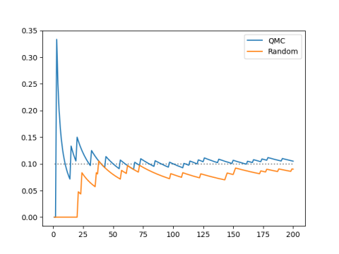
The horizontal axis is the length of the sequence and the vertical axis is the proportion of sequence elements that fall into the test interval.
Our sequence spends about 1/10 of its time in this interval of length 1/10. The same is true of a random sequence, eventually, and with high probability. Our sequence achieves the limiting behavior of a random sequence, but it achieves it more quickly, and it does so with certainty, not just with high probability.
Here’s another example just to show that our initial choice of interval didn’t matter. We use the interval
[π − 3, e − 2] = [0.141…, 0.718…]
and we get analogous results.
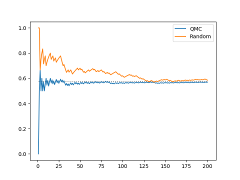
The interval has width 0.57, and our sequence spends 57% of its time in the interval.
Quasi-Monte Carlo and low discrepancy
Our sequence is an example of a Quasi-Monte Carlo (QMC) sequence. The name implies that the sequence is something like a random sequence, but better in some sense. QMC sequences are said to have low discrepancy, meaning that the difference (discrepancy) between the number of points that land in an interval and the expected number is low, lower than what you’d expect from a random (Monte Carlo) sequence.
To define discrepancy rigorously we get rid of our arbitrary choice of interval and take the supremum over all subintervals. Or we could define the star-discrepancy by taking the supremum over subintervals that must start with 0 on the left end.
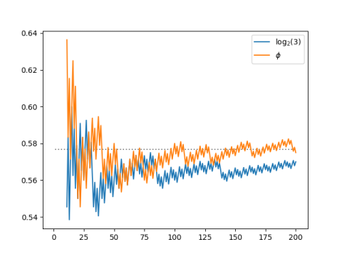
Even lower discrepancy
It turns out we could do better with a different choice of k. For any irrational k the sequence
kn mod 1
has low discrepancy, i.e. lower than you’d expect from a random sequence, but the discrepancy is as small as possible when k is the golden ratio.
Application
We’ve been looking at a QMC sequence in an interval, but QMC sequences in higher dimension are defined analogously. In any volume of space, the visits the space more uniformly than a random sequence.
QMC sequences are usually applied in higher dimensions, and the primary application is numerical integration. Quasi-Monte Carlo integration is more efficient than Monte Carlo integration, though the error is harder to estimate; QMC integration often does better in practice than pessimistic theoretical bounds predict. A hybrid of QMC and MC can retain the efficiency of QMC and a some of the error estimation of MC.
See more on QMC sequences are used in numerical integration.
I’ve always been a big fan of the Sobol sequence and tend to use that in most cases.
For low dimensions the golden ratio trick works really well but I have found that there are weird underlying patterns in the points chosen. They may pass the discrepancy test as the number of points heads to infinity, but if you show a plot to a customer they often get distracted with the patterns that show up. And sometimes the customer management matters too :)
One of my favorite ways of doing this is to use powers of the golden ratio for the dimensions. That is, the quasirandom choice for coordinate x_i is phi^i*n mod 1
“To define discrepancy rigorously we get rid of our arbitrary choice of interval and take the supremum over all subsets of the interval with positive measure.”
Am I missing something? Every sequence is countable, so “the set of points in [0, 1] not visited by our sequence” has measure 1, but 0% of the points in the sequence land in it. Or does this apply to families of sequences rather than individual sequences?
Nathan, you’re right: I made a mistake in describing the definition. I edited the post to correct it.