Yesterday I wrote about how to interpolate a Brownian path. If you’ve created a discrete Brownian path with a certain step size, you can go back and fill in at smaller steps as if you’d generated the values from the beginning.
This means that instead of generating samples in order as a random walk, you could generate the samples recursively. You could generate the first and last points, then fill in a point in the middle, then fill in the points in the middle of each subinterval etc. This is very much like the process of creating a Cantor set or a Koch curve.
In Brownian motion, the variance of the difference in the values at two points in time is proportional to the distance in time. To step forward from your current position by a time t, add a sample from a normal random variable with mean 0 and variance t.
Suppose we want to generate a discrete Brownian path over [0, 128]. We could start by setting W(0) = 0, then setting W(1) to a N(0, 1) sample, then setting W(2) to be W(1) plus a N(0, 1) sample etc.
The following code carries this process out in Python.
    import numpy as np

    N = 128
    W = np.zeros(N+1)
    for i in range(N):
        W[i+1] = W[i] + np.random.normal()
We could make the code more precise, more efficient, but less clear [1], by writing
W = np.random.normal(0, 1, N+1).cumsum()
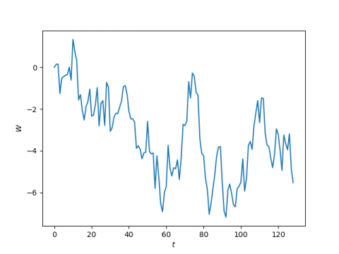
In either case, here’s a plot of W.
But if we want to follow the fractal plan mentioned above, we’d set W(0) = 0 and then generate W(128) by adding a N(0, 128) sample. (I’m using the second argument in the normal distribution to be variance. Conventions vary, and in fact NumPy’s random.gaussian takes standard deviation rather than variance as its second argument.)
    W[0] = 0
    W[128] = np.random.gaussian(0, 128**0.5)
Then as described in the earlier post, we would generate W(64) by taking the average of W(0) and W(128) and adding a N(0, 32) sample. Note that the variance in the sample is 32, not 64. See the earlier post for an explanation.
W[64] = 0.5*(W[0] + W[128]) + np.random.gaussian(0, 32**0.5)
Next we would fill in W(32) and W(96). To fill in W(32) we’d start by averaging W(0) and W(64), then add a N(0, 16) sample. And to fill in W(96) we’d average W(64) and W(128) and add a N(0, 16) sample.
    W[32] = 0.5*(W[0]  + W[64] ) + np.random.gaussian(0, 16**0.5)
    W[96] = 0.5*(W[64] + W[128]) + np.random.gaussian(0, 16**0.5)
We would continue this process until we have samples at 0, 1, 2, …, 128. We won’t get the same Brownian path that we would have gotten if we’d sampled the paths in order—this is all random after all—but we’d get an instance of something created by the same stochastic process.
To state the fractal property explicitly, if W(t) is a Brownian path over [0, T], then
W(c² T)/c
is a Brownian path over [0, c² T]. Brownian motion looks the same at all scales.
***
The “less clear” part depends on who the reader is. The more concise version is more clear to someone accustomed to reading such code. But the loop more explicitly reflects the sequential nature of constructing the path.