Rate of natural cubic spline convergence

Suppose you want to approximate a function with a polynomial by interpolating it at evenly spaced points. You might reasonably expect that the more points you use, the better the approximation will be. That might be true, but it might not. As explained here, for some functions the maximum approximation error actually increases as the number of points increases. This is called the Runge phenomenon.

What about cubic splines? Instead of fitting one high-degree polynomial, you fit a different cubic polynomial on each sub-interval, with the constraint that the pieces fit together smoothly. Specifically, the spline must be twice differentiable. This means that the first and second derivatives from both sides match at the end of each interval.

Say our function f is defined over an interval [a, b] and we break the interval into n sub-intervals. This means we interpolate f at n+1 evenly spaced points. We have 4n degrees of freedom: four polynomial coefficients over each interval. Interpolation adds 2n constraints: the value of the polynomial is specified at the ends of each sub-interval. Matching first and second derivatives at each of the n-1 interior nodes gives 2(n-1) constrains. This is a total of 4n – 2 equations for 4n unknowns.

We get the two more equations we need by specifying something about the derivatives at a and b. A natural cubic spline sets the second derivatives equal to zero at a and b.

So if we interpolate f at n+1 evenly spaced points using a natural cubic spline, does the splines converge uniformly to f as we increase n? Indeed they do. Nothing like Runge phenomenon can happen. If f is four times continuously differentiable over [a, b], then convergence is uniform on every compact subinterval of (a, b) and the rate of convergence is O(1/n⁴). If the second derivative of f is zero at a and b, then the rate of convergence is O(1/n⁴) over the whole interval [a, b].

Source: Kendall E. Atkinson. On the Order of Convergence of Natural Cubic Spline Interpolation. SIAM Journal on Numerical Analysis, Vol. 5, No. 1 (Mar., 1968), pp. 89-101.

Update: See this post for results for other kinds of cubic splines, i.e. cubic splines with different boundary conditions.

Experiment

We will look at sin(x) and exp(x) on the interval [0, 2π]. Note that the second derivatives of former at zero at both ends of the interval, but this is not true for the latter.

We will look at the error when interpolating our functions at 11 points and 21 points (i.e. 10 sub-intervals and 20 sub-intervals) with natural cubic splines. For the sine function we expect the error to go down by about a factor of 16 everywhere. For the exponential function, we expect the error to go down by about a factor of 16 in the interior of [0, 2π]. We’ll see what happens when we zoom in on the interval [2, 4].

We’re basing our expectations on a theorem about what happens as the number of nodes n goes to infinity, and yet we’re using fairly small values of n. So we shouldn’t expect too close of an agreement with theory, but we’ll see how close our prediction gets.

Computation

The following Python code will plot the error in the interpolation by natural cubic splines.

    import numpy as np
    from scipy.interpolate import CubicSpline
    import matplotlib.pyplot as plt

    for n in [11, 21]:
        for f in [np.sin, np.exp]:
            knots = np.linspace(0, 2*np.pi, n)
            cs = CubicSpline(knots, f(knots))
            x = np.linspace(0, 2*np.pi, 200)
        
            plt.plot(x, f(x) - cs(x))
            plt.xlabel("$x$")
            plt.ylabel("Error")
            plt.title(f"Interpolating {f.__name__} at {n} points")
            plt.savefig(f"{f.__name__}_spline_error_{n}.png")
            plt.close()

Notice an interesting feature of NumPy: we call the __name__ method on sin and exp to get their names as strings to use in the plot title and in the graphic file.

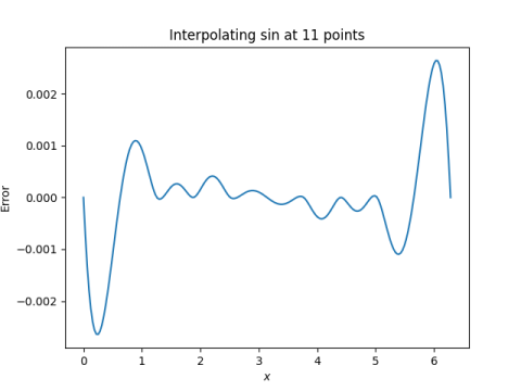
Here’s what we get for the sine function.

First for 10 intervals:

Then for 20 intervals:

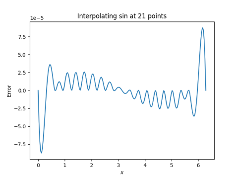
When we doubled the number of intervals, the maximum error went down by about 30x, better than the theoretical upper bound on error.

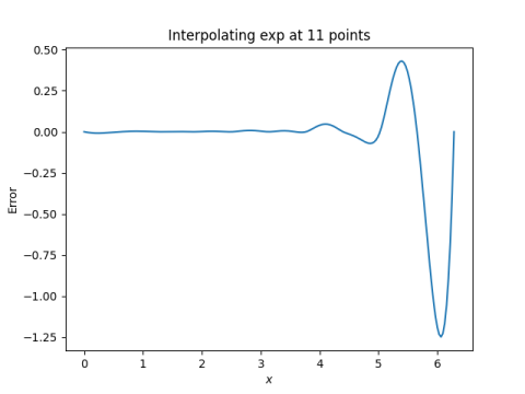
Here’s what we get for the exponential function.

First for 10 intervals:

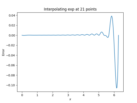
Then for 20 intervals:

The error in approximating the exponential function by splines is much greater than the error in approximating the sine function. That’s because the former acts less like a polynomial than the latter. Polynomial approximation, and piecewise polynomial approximation, works better on things that behave like polynomials.

When we doubled the number of intervals, the maximum error went down by a factor of 12. We shouldn’t be surprised that the error to go down by a factor of less than 16 since the hypotheses for the theorem that gives a factor of 16 aren’t satisfied.

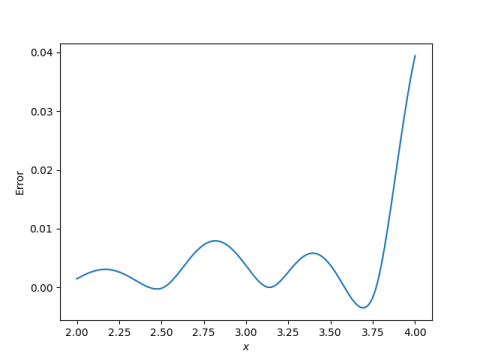
Here’s what we get when we zoom in on the interval [2, 4].

For 10 subintervals:

And for 20 subintervals:

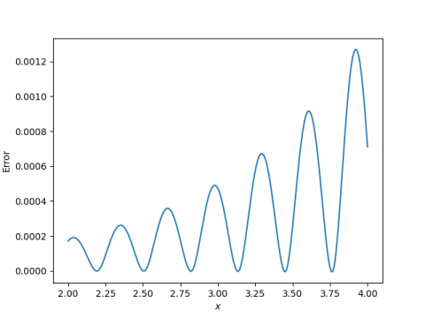
The error is much smaller over the interior interval. And when we double the number of interpolation points, the error over [2, 4] goes down by about a factor of 3 just as it did for sine.

Note that in these last two plots, we’re still interpolating over the entire interval [0, 2π], but we’re looking at the error over [2, 4]. We’re zooming in on part of the error plot, not allocating our interpolation points specifically to the smaller interval.

Related posts

• Chebyshev interpolation
• Monotonic interpolation