Solutions to the non-linear differential equation
x ″ + 0.25x ′ + x(x² − 1) = 0.3 cos t
are chaotic. It’s more common to see plots of chaotic systems in the time domain, so I wanted to write a post looking at the power spectrum in the frequency domain.
The following plot was created by solving the equation above over the time interval [0, 256] at 1024 points, i.e. sampling the solution at 4 Hz. I then took the FFT and multiplied it by its conjugate to get the power spectrum. Then I took the log base 10 and multiplied by 10 to convert to decibels.
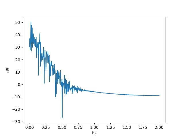
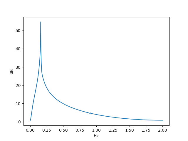
By contrast, if we look at the linear equation
x ″ + 0.25x ′ + x = 0.3 cos t
and compute the power spectrum, we get
As is often the case, a small change to the form of a differential equation made a huge change in its behavior.
There’s a spike at 1/2π Hz because the steady-state solution is
x(t) = 1.2 sin(t).
The power spectrum is more than just a spike because there is also an exponentially decaying transient component to the solution.
For more on steady-state and transient components of the solution, see Damped, driven oscillations.
In the power spectrum graph there seems to be a tiny oscilation at 0.9 Hz. Any explanation?
Funny typo at the end: Predatory.
It sorta makes sense that there are no high-frequency components, because the nonlinear term is approximately linear over short intervals, but other than that, it’s hard to say why the spectrum is what it is.