The last several posts have been looking at the bifurcation diagram below in slices.
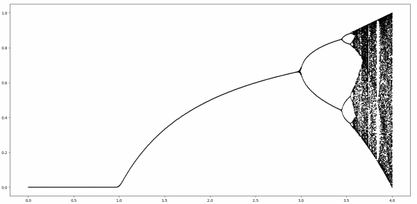
The first post looked at the simple part, corresponding to the horizontal axis r running from 0 to 3.
The next post looked at the first fork, for r between 3 and 3.4495.
The previous post looked at the period doubling region, for r between 3.4495 and 3.56995.
For r greater than about 3.56995 we enter the chaotic region. This post looks at an apparent island of stability inside the chaotic region. This island starts at r = 1 + √8 = 3.8284.
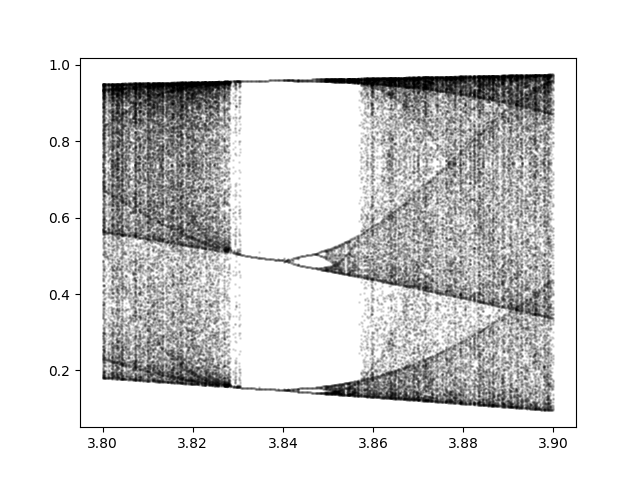
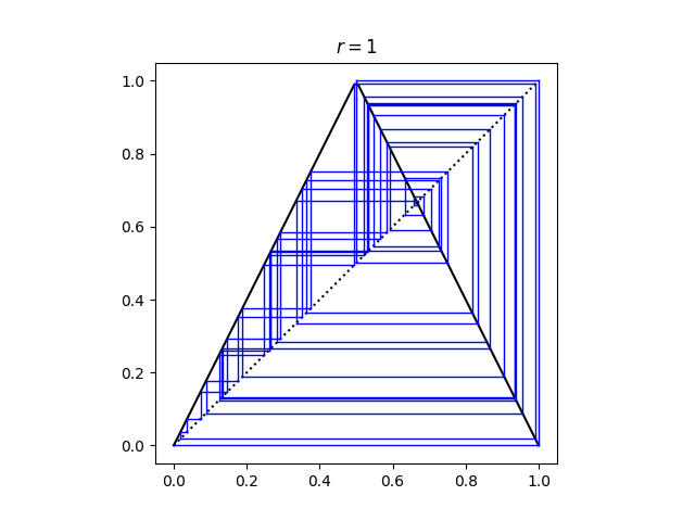
The whitespace indicates an absence of stable cycle points. There are unstable cycle points, infinitely many in fact, as we will soon see. For a small range of r there are three stable cycle points. When r = 3.83, for example, the three cycle points are 0.1561, 0.5047, and 0.9574.
This is significant because period three implies chaos. There is a remarkable theorem that says if a continuous map of a bounded interval to itself has a point with period 3, then it also has points with periods 4, 5, 6, … as well as an uncountable number of points with no period. If there are points with period 4, why can’t we see them? Because they’re unstable. You would have to land exactly on one of these points to go in a cycle. If you’re off by the tiniest amount, which you always are in computer arithmetic, you won’t stay in the cycle.
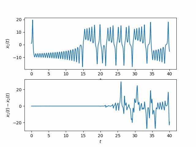
So even when we’re in the region with three stable points, things are still technically chaotic.
There seems to be something paradoxical about computer demonstrations of chaos. If you have extremely sensitive dependence on initial conditions, how can floating point operations, which are not exact, demonstrate chaos? I would say they can illustrate chaos rather than demonstrate chaos. And sometimes you can do computer calculations which do not have such sensitivity to show that other things are sensitive.
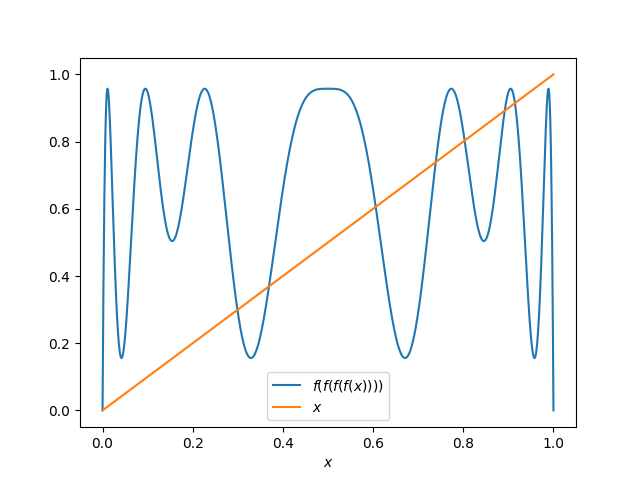
For example, I asserted above that there are points with period 4. Let f be the logistic map with r = 3.83
f(x) = 3.83 x(1 − x)
and define
p(x) = f(f(f(f(x)))),
i.e. four applications of f. Then you can see that there must be a point with period 4 because the graph of p(x) crosses the graph of x.
So while our region of whitespace appears to be empty except for three stable cycle points, there are infinitely many more cyclic points scattered like invisible dust in the region, a set of measure zero that we cannot see.