Random Blaschke products and Mathematica binding

A Blaschke product is a function that is the product of Blaschke factors, functions of the form

b(z; a) = |a|  (a – z) / a (1 – a*z)

where the complex number a lies inside the unit circle and a* is the complex conjugate of a.

I wanted to plot Blaschke products with random values of a using Mathematica, and I ran into a couple items of interest.

First, although Mathematica has a function RandomComplex for returning complex numbers chosen by a pseudorandom number generator, this function selects complex numbers uniformly over a rectangle and I wanted to select uniformly over a disk. This is easy enough to get around. I wrote my own function by selecting a magnitude and phase at random.

    rc[] := Sqrt[RandomReal[]] Exp[-2 Pi I RandomReal[]]

Now if I reuse the definition of a Blaschke factor from an earlier post

    b[z_, a_] := (Abs[a]/a) (a - z)/(1 - Conjugate[a] z)

I can define a product of two random Blaschke factors as follows.

    f[z_] := b[z, rc[]]  b[z, rc[]]

However, this may not do what you expect. If you plot the function twice, you’ll get different results! It’s a matter of binding order. At what point in the process are the two random values of a chosen and fixed? The answer is some time between the definition of f and executing the plotting function. If the plotting function generated new values of a every time it needed to evaluate f the result would be a hot mess.

On the other hand, if we leave out the colon then the function f behaves as expected.

    f[z_] = b[z, rc[]]  b[z, rc[]]

Now random values are generated by each call to rc, and these values are frozen in the definition of f.

Here’s a Blaschke product with 10 random parameters.

    f[z_] = Product[b[z, rc[]], {i, 1, 10}]

The code

    ComplexPlot[f[z], {z, -1 - I, 1 + I}]

produces the following plot.

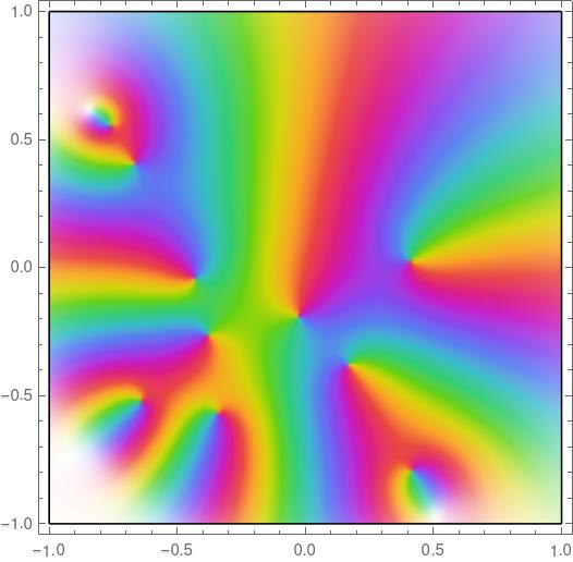
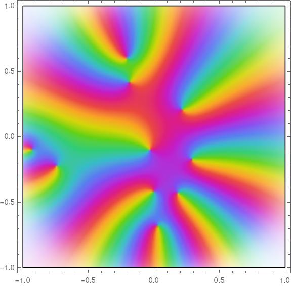
If I plot this function again, say changing the plot range, I’ll plot the same function. But if I execute the line of code defining f again, and call ComplexPlot again, I’ll generate a new function.

Incidentally, if I plot this same function using ComplexPlot3d I get the following.

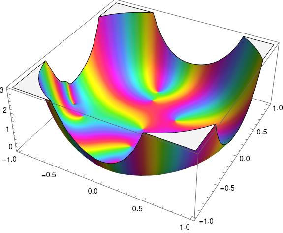
Why does it look like a bowl? As explained in the post on Blaschke factors, each factor is zero at its parameter a and has a pole at the reflection of a in the unit disk.

The function plotted above has zeros inside the unit disk near the boundary. That means it also has poles outside the unit disk near the boundary on the other side.