Numerically evaluating a theta function

Theta functions pop up throughout pure and applied mathematics. For example, they’re common in analytic number theory, and they’re solutions to the heat equation.

Theta functions are analogous in some ways to trigonometric functions, and like trigonometric functions they satisfy a lot of identities. This post will comment briefly on an identity that makes a particular theta function, θ₃, easy to compute numerically. And because there are identities relating the various theta functions, a method for computing θ₃ can be used to compute other theta functions.

The function θ₃ is defined by

$\theta_3(z, t) = 1 + \sum_{k=1}^\infty q^{k^2} \cos(2kz)$

where

$q = e^{\pi i t}$

Here’s a plot of θ₃ with t = 1 + i

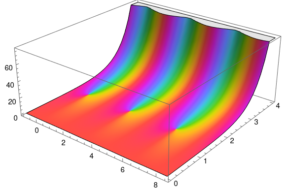
produced by the following Mathematica code:

    
    q = Exp[Pi I (1 + I)]
    ComplexPlot3D[EllipticTheta[3, z, q], {z, -1, 8.5 + 4 I}]

An important theorem tells us

$\theta_3(z, t) = (-it)^{-1/2} \exp(z^2/\pi i t)\, \theta_3\left(\frac{z}{t}, -\frac{1}{t} \right )$

This theorem has a lot of interesting consequences, but for our purposes note that the identity has the form

$\theta_3(\ldots, t) = \ldots \theta_3\left(\ldots, -\frac{1}{t} \right )$

The important thing for numerical purposes is that t is on one side and 1/t is on the other.

Suppose t = a + bi with a > 0 and b > 0. Then

$q = \exp\left(\pi i (a + bi)\right) = \exp(-\pi b) \exp(\pi i a)$

Now if b is small, |q| is near 1, and the series defining θ₃ converges slowly. But if b is large, |q| is very small, and the series converges rapidly.

So if b is large, use the left side of the theorem above to compute the right. But if b is small, use the right side to compute the left.

Related posts