I wrote a while back about the function
f(t) = arctan(k tan(t)).
I keep running into this function. Has anybody given this function a name or studied it?
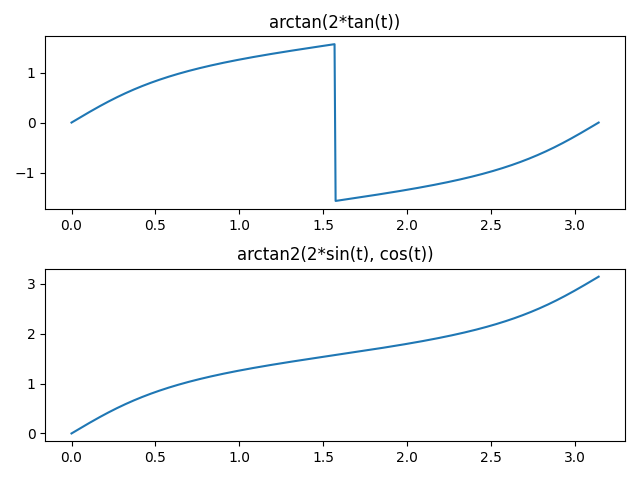
The direct implementation has a discontinuity at π/2 but I needed to extend it continuously. Using the two-argument version of inverse tangent fixes this. In Python, the implementation is
arctan2(k*sin(t), cos(t))
Here are plots of the direct and improved version.
Mathematica does not have a function ArcTan2. Instead, it overloads the ArcTan function to take either one or two arguments. But beware: the two-argument version of ArcTan in Mathematica takes its arguments in the opposite order of functions like atan2 in C.
This extends the continuous range from [0, π/2] to [0, π], but there’s still a discontinuity at π. The trick to extending further is to reduce the argument mod π, subtract off the reduced argument, then add the original argument back in. In Python:
arctan2(k*sin(t%pi), cos(t%pi)) - t%pi + t
This plot shows the extension works.
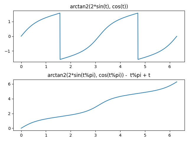
Now the function extends smoothly to the entire real line.
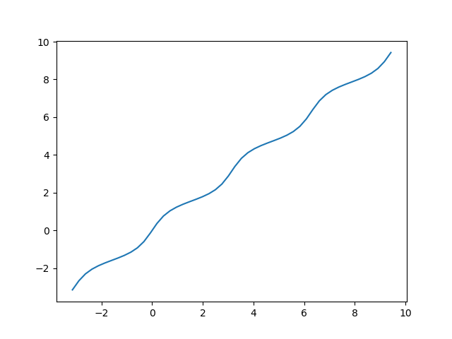
Here’s a Mathematica implementation of the smooth extension.
g[x_, k_] := Module[{y = Mod[x, Pi]}, ArcTan[Cos[y], k Sin[y]] - y + x]
The function g(x, k) is an increasing function of x for fixed k ≠ 0, and its inverse is the same function replacing k with 1/k:
g( g(x, 1/k), k ) = x.
Here’s a plot of the function g with the linear trend subtracted, letting k vary from 1 to 10.
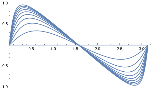
This was made with the following code.
Plot[Table[g[x, n] - x, {n, 1, 10}], {x, 0, Pi}]
As k increases, the amplitude increases, and the peaks move away from the center. You can confirm this by taking the derivative. The maximum occurs at arccos(√(k/(k+1))) and so the maxima locations converge to 0 as k → ∞. By symmetry the minima locations converge to π.You can also verify that the maximum value is arctan(√k), and so the maxima converge to π/2, and by symmetry the minima converge to -π/2;.
This plot looks similar to the plot of true anomaly for a highly elliptical orbit. I’m sure they’re related, but I haven’t worked out exactly how.
If we add back in the linear trend that we’d subtracted off, we see that for large k, g(x, k) is a smooth approximation to a stairstep function, analogous to the soft maximum function.
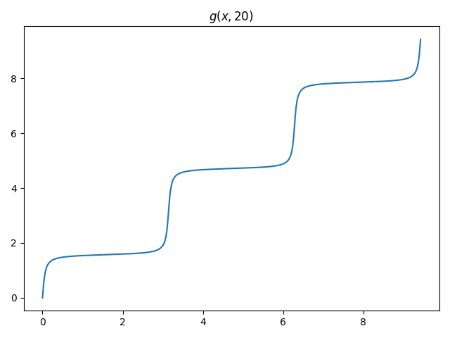

You could just add the appropriate “staircase” function to get the continuous extension:
g[x_, k_] := ArcTan[k Tan[x]] + Pi Floor[x/Pi + 1/2]