Edmond Laguerre (1834–1886) came up with a method for finding zeros of polynomials. Unlike Newton’s method for finding zeros of general functions, Laguerre’s method is specialized for polynomials. Laguerre’s method converges an order of magnitude faster than Newton’s method, i.e. the error is cubed on each step rather than squared.
The most interesting thing about Laguerre’s method is that it nearly always converges to a root, no matter where you start. Newton’s method, on the other hand, converges quickly if you start sufficiently close to a root. If you don’t start close enough to a root, the method might cycle or go off to infinity.
The first time I taught numerical analysis, the textbook we used began the section on Newton’s method with the following nursery rhyme:
There was a little girl,
Who had a little curl,
Right in the middle of her forehead.
When she was good,
She was very, very good,
But when she was bad, she was horrid.
When Newton’s method is good, it is very, very good, but when it is bad it is horrid.
Laguerre’s method is not well understood. Experiments show that it nearly always converges, but there’s not much theory to explain what’s going on.
The method is robust in that it is very likely to converge to some root, but it may not converge to the root you expected unless you start sufficiently close. The rest of the post illustrates this.
Let’s look at the polynomial
p(x) = 3 + 22x + 20x² + 24x³.
This polynomial has roots at 0.15392, and at -0.3397 ± 0.83468i.
We’ll generate 2,000 random starting points for Laguerre’s method and color its location according to which root it converges to. Points converging to the real root are colored blue, points converging to the root with positive imaginary part are colored orange, and points converging to the root with negative imaginary part are colored green.
Here’s what we get:
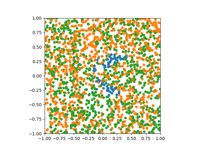
This is hard to see, but we can tell that there aren’t many blue dots, about an equal number of orange and green dots, and the latter are thoroughly mixed together. This means the method is unlikely to converge to the real root, and about equally likely to converge to either of the complex roots.
Let’s look at just the starting points that converge to the real root, its basin of attraction. To get more resolution, we’ll generate 100,000 starting points and make the dots smaller.
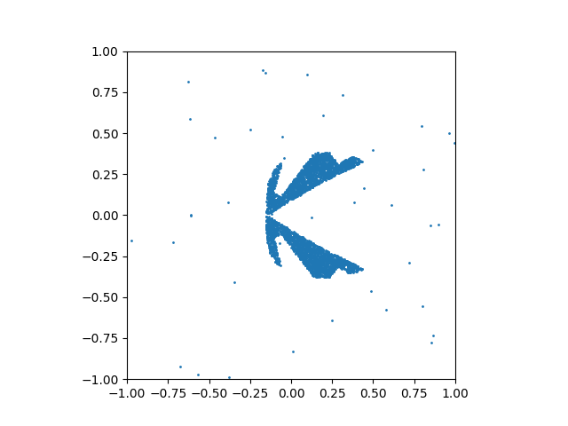
The convergence region is pinched near the root; you can start fairly near the root along the real axis but converge to one of the complex roots. Notice also that there are scattered points far from the real root that converge to that point.
Next let’s look at the points that converge to the complex root in the upper half plane.
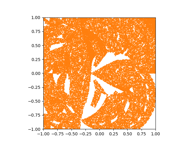
Note that the basin of attraction appears to take up over half the area. But the corresponding basin of attraction for the root in the lower half plane also appears to take up over half the area.
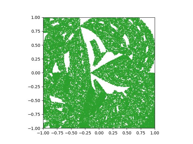
They can’t both take up over half the area. In fact. both take up about 48%. But the two regions are very intertwined. Due to the width of the dots used in plotting, each green dot covers a tiny bit of area that belongs to orange, and vice versa. That is, the fact that both appear to take over half the area shows how commingled they are.
I think there is a bug in your Laguerre’s method. When I initially implemented mine using numpy, I had used `numpy.maximum(gp, gm)` to pick the sign on the radical in the denominator, and saw the beautiful fractal patterns you see. However, this is a bug, because the radical takes a complex value, so `numpy.maximum` is picking the value with the largest real part, rather than the largest absolute value. When I switched to using `np.where(np.abs(gp) > np.abs(gm), gp, gm)`, the fractal patterns disappeared, replaced by very regular basins of attraction.