The Poisson probability distribution gives a simple, elegant model for count data. You can even derive from certain assumptions that data must have a Poisson distribution. Unfortunately reality doesn’t often go along with those assumptions.
A Poisson random variable with mean λ also has variance λ. But it’s often the case that data that would seem to follow a Poisson distribution has a variance greater than its mean. This phenomenon is called over-dispersion: the dispersion (variance) is larger than a Poisson distribution assumption would allow.
One way to address over-dispersion is to use a negative binomial distribution. This distribution has two parameters, r and p, and has the following probability mass function (PMF).
As the parameter r goes to infinity, the negative binomial distribution converges to a Poisson distribution. So you can think of the negative binomial distribution as a generalization of the Poisson distribution.
These notes go into the negative binomial distribution in some detail, including where its name comes from.
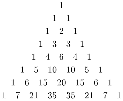
If the parameter r is a non-negative integer, then the binomial coefficients in the PMF for the negative binomial distribution are on the (r+1)st diagonal of Pascal’s triangle.

The case r = 0 corresponds to the first diagonal, the one consisting of all 1s. The case r = 1 corresponds to the second diagonal consisting of consecutive integers. The case r = 2 corresponds to the third diagonal, the one consisting of triangular numbers. And so forth.
