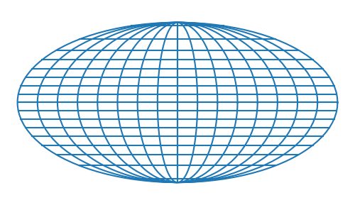
Karl Brandan Mollweide (1774-1825) designed an equal-area map projection, mapping the surface of the earth to an ellipse with an aspect ratio of 2:1. If you were looking at the earth from a distance, the face you’re looking at would correspond to a circle in the middle of the Mollweide map [1]. The part of the earth that you can’t see is mapped to the rest of the ellipse.
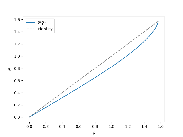
The lines of latitude are not quite evenly spaced; some distortion is required to achieve equal area. Instead, latitude φ corresponds to θ on the map according to the equation
![]()
There is no closed-form solution for θ as a function of φ and so the equation must be solved numerically. For each φ we have to find the root of
![]()
Here’s a plot of θ as a function of φ.
Newton’s method
Newton’s method works efficiently (converges quadratically) except when φ is close to π/2. The reason Newton’s method slows down for high latitudes is that f and its derivative are both at π/2, i.e. f has a double root there.
Newton’s method slows down from quadratic to linear convergence near a double root, but there is a minor modification that maintains quadratic convergence near a double root.
![]()
When m = 1 this is the usual form of Newton’s method. Setting m = 2 tunes the method for double roots.
The modified version of Newton’s method with m = 2 works when the root you’re trying to is exactly a double root. However, if you’re trying to find a root near a double root, setting m = 2 can cause the method to diverge, so you have to be very careful with changing m.
Illustration
Here’s a version of Newton’s method, specialized for the Mollweide equation. We can specify the value of m, and the initial estimate of the root defaults to θ = φ.
from numpy import sin, cos, pi

def mynewton(phi, m, x0 = None):
    x = x0 if x0 else phi
    delta = 1
    iterations = 0

    while abs(delta) > 1e-12:
        fx = 2*x + sin(2*x) - pi*sin(phi)
        fprime = 2 + 2*cos(2*x)
        delta = m*fx/fprime
        x -= delta
        iterations += 1

    return (x, iterations)
Far from the double root
Say φ = 0.25 and m = 1. When we use the default initial estimate Newton’s method converges in 5 iterations.
Near the double root
Next, say φ = π/2 − 0.001. Again we set m = 1 and use the default initial estimate. Now Newton’s method takes 16 iterations. The convergence is slower because we’re getting close to the double root at π/2.
But if we switch to m = 2, Newton’s method diverges. Slow convergence is better than no convergence, so we’re better off sticking with m = 1.
On the double root
Now let’s say φ = π/2. In this case the default guess is exactly correct, but the code divides by zero and crashes. So let’s take our initial estimate to be π/2 − 0.001. When m = 1, Newton’s method takes 15 steps to converge. When m = 2, it converges in 6 steps, which is clearly faster. However, both cases the returned result is only good to 6 decimal places, even though the code is looking for 12 decimal places.
This shows that as we get close to φ = π/2, we have both a speed and an accuracy issue.
A better method
I haven’t worked this out, but here’s how I imagine I would fix this. I’d tune Newton’s method, preventing it from taking steps that are too large, so that the method is accurate for φ in the range [0, π/2 − ε] and use a different method, such as power series inversion, for φ in [π/2 − ε, π/2].
Update: The next post works out the series solution alluded to above.
Related posts
- Inverse Mercator projection
- Equal Earth map projection
- Solving Kepler’s equation with Newton’s method
[1] Someone pointed out on Hacker News that this statement could be confusing. The perspective you’d see from a distance is not the Mollweide projection—that would not be equal area—but it corresponds to the same region. As someone put it on HN “a circle in the center corresponds to one half of the globe.”