A closer look at Cosh[ArcCosh[x] + ArcCosh[y]]

The previous post derived the identity

$\cosh\Big( \operatorname{arccosh}(x) + \operatorname{arccosh}(y)\Big) = xy + \sqrt{x^2 -1} \sqrt{y^2 -1}$

and said in a footnote that the identity holds at least for x > 1 and y > 1. That’s true, but let’s see why the footnote is necessary.

Let’s have Mathematica plot

$\left| \cosh\Big( \operatorname{arccosh}(x) + \operatorname{arccosh}(y)\Big) - xy - \sqrt{x^2 -1} \sqrt{y^2 -1} \right|$

The plot will be 0 where the identity above holds.

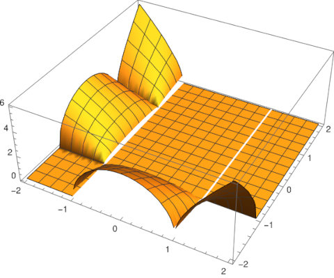
The plot is indeed flat for x > 1 and y > 1, and more, but not everywhere.

If we combine the two square roots

$\left| \cosh\Big( \operatorname{arccosh}(x) + \operatorname{arccosh}(y)\Big) - xy - \sqrt{(x^2 -1) (y^2 -1)} \right|$

and plot again we still get a valid identity for x > 1 and y > 1, but the plot changes.

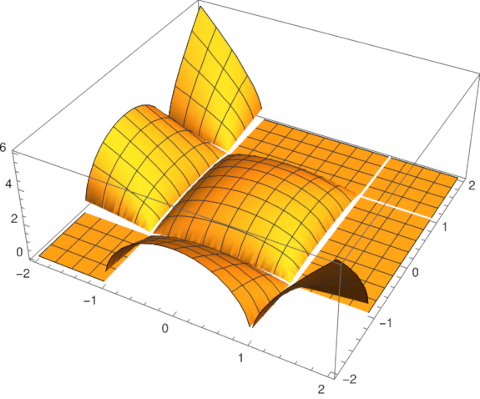
This is because √a √b does not necessarily equal √(ab) when the arguments may be negative.

The square root function and the arccosh function are not naturally single-valued functions. They require branch cuts to force them to be single-valued, and the two functions require different branch cuts. I go into this in some detail here.

There is a way to reformulate our identity so that it holds everywhere. If we replace

$\sqrt{z^2 - 1}$

with

$f(z) = \exp\left( \tfrac{1}{2}\left( \log(z - 1) + \log(z + 1) \right) \right)$

which is equivalent for z > 1, the corresponding identity holds everywhere.

We can verify this with the following Mathematica code.

f[z_] := Exp[(1/2) (Log[z - 1 ] + Log[z + 1])]
FullSimplify[Cosh[ArcCosh[x] + ArcCosh[y]] - x y - f[x] f[y]]

This returns 0.

By contrast, the code

FullSimplify[
 Cosh[ArcCosh[x] + ArcCosh[y]] - x y - Sqrt[x^2 - 1] Sqrt[y^2 - 1]]

simply returns its input with no simplification, unless we add restrictions on x and y. The code

FullSimplify[
 Cosh[ArcCosh[x] + ArcCosh[y]] - x y - Sqrt[x^2 - 1] Sqrt[y^2 - 1], 
 Assumptions -> {x > -1 && y > -1}]

does return 0.

Closer look at an identity

Related posts

Leave a Reply