Here’s a simple calculation that I’ve done often enough that I’d like to save the result for my future reference and for the benefit of anyone searching on this.

A linear combination of sines and cosines

a sin(x) + b cos(x)

can be written as a sine with a phase shift

A sin(x + φ).

Going between {a, b} and {A, φ} is the calculation I’d like to save. For completeness I also include the case

A cos(x + ψ).

Derivation

Define

f(x) = a sin(x) + b cos(x)

and

g(x) = A sin(x + φ).

Both functions satisfy the differential equation

y″ + y = 0

and so f = g if and only if f(0) = g(0) and f′(0) = g′(0).

Setting the values at 0 equal implies

b = A sin(φ)

and setting the derivatives at 0 equal implies

a = A cos(φ).

Taking the ratio of these two equations shows

b/a = tan(φ)

and adding the squares of both equations shows

a² + b² = A².

Equations

First we consider the case

a sin(x) + b cos(x) = A sin(x + φ).

Sine with phase shift

If a and b are given,

A = √(a² + b²)

and

φ = tan⁻¹(b / a).

If A and φ are given,

a = A cos(φ)

and

b = A sin(φ)

from the previous section.

Cosine with phase shift

Now suppose we want

a sin(x) + b cos(x) = A cos(x + ψ)

If a and b are given, then

A = √(a² + b²)

as before and

ψ = − tan⁻¹(a / b).

If A and ψ are given then

a = − A sin(ψ)

and

b = A cos(ψ).

Related posts

• Convert between real and complex Fourier series
• Converting between error function and normal CDF [pdf]
• Converting trig identities to hyperbolic identities
• Technical notes

I recently stumbled upon the Postage Stamp Problem. Given two relatively prime positive numbers a and b, show that any sufficiently large number N, there exists nonnegative integers x and y such that

ax + by = N.

I initially missed the constraint that x and y must be positive, in which result is well known (Bézout’s lemma) and there’s no requirement for N to be large. The positivity constraint makes things more interesting.

The problem is called the Postage Stamp Problem because it says that given any two stamps whose values are relatively prime, say a 5¢ stamp and a 21¢ stamp, you can make any sufficiently large amount of postage using just those two stamps.

A natural question is how large is “sufficiently large,” and the answer turns out to be all integers larger than

ab − a − b.

So in our example, you cannot make 79¢ postage out of 5¢ and 21¢ stamps, but you can make 80¢ or any higher amount.

If you’ve been reading this blog for a while, you may recognize this as a special case of the Chicken McNugget problem, which you can think of as the Postage Stamp problem with possibly more than two stamps.

Related posts

• The Chicken McNugget monad
• Cicadas and chicken nuggets
• Possible and actual football scores

It’s easier to go up a ladder than to come down, literally and metaphorically.

Gian-Carlo Rota made a profound observation on the application of theory.

One frequently notices, however, a wide gap between the bare statement of a principle and the skill required in recognizing that it applies to a particular problem.

This isn’t quite what he said. I made two small edits to generalize his actual statement. He referred specifically to the application of the inclusion-exclusion principle to problems in combinatorics. Here is his actual quote from [1].

One frequently notices, however, a wide gap between the bare statement of the principle and the skill required in recognizing that it applies to a particular combinatorial problem.

This post will expand a little on Rota’s original statement and a couple applications of the more general version of his statement.

The inclusion-exclusion principle

I don’t think Rota would have disagreed with my edited version of his statement, but it’s interesting to think of his original context. The inclusion-exclusion principle seems like a simple problem solving strategy: you may count a set of things by first over-counting, then correcting for the over-counting.

For example, a few days ago I wrote about a graph created by turning left at the nth step if n is divisible by 7 or contains a digit 7. Suppose you wanted to count how many times you turn in the first 100 steps. You could count the number of positive integers up to 100 that are divisible by 7, then the number that contain the digit 7, then subtract the number that both are divisible by 7 and contain a 7.

You can carry this a step further by over-counting, then over-correcting for your over-counting, then correcting for your over-correction. This is the essence of the following probability theorem.

The inclusion-exclusion principle a clever idea, but not that clever. And yet Rota discusses how this idea was developed over decades into the Möbius inversion principle, which has diverse applications, including Euler characteristic and the calculus of finite differences.

Bayes’ theorem

Bayesian statistics is a direct application of Bayes’ theorem. Bayes’ theorem is a fairly simple idea, and yet people make careers out of applying it.

When I started working in the Biostatistics Department at MD Anderson, a bastion of Bayesian statistics, I was surprised how subtle Bayesian statistics is. I probably first saw Bayes’ theorem as a teenager, and yet it was not easy to wrap my head around Bayesian statistics. I would think “This is simple. Why is this hard?” The core principle was simple, but the application was not trivial.

Newtonian mechanics

When I took introductory physics, we would get stuck on homework problems and ask our professor for help. He would almost always begin by saying “Well, F = ma.”

This was infuriating. Yes, we know F = ma. But how does that let us solve this problem?!

There’s more to Newtonian mechanics than Newton’s laws, a lot more. And most of it is never made explicit. You pick it up by osmosis after you’ve worked hundreds of exercises.

Related posts

• There’s more going on here
• Applied abstraction

[1] G. C. Rota. On the Foundations of Combinatorial Theory I. Theory of Möbius Functions. Z. Wahrscheinlichkeitstheorie und Verw. Gebiete, 2 (1964) 340–368.

I learned to use the command line utility make in the context of building C programs. The program make reads an input file to tell it how to make things. To make a C program, you compile the source files into object files, then link the object files together.

You can tell make what depends on what, so it will not do any unnecessary work. If you tell it that a file foo.o depends on a file foo.c, then it will rebuild foo.o if that file is older than the file foo.c that it depends on. Looking at file timestamps allows make to save time by not doing unnecessary work. It also makes it easier to dictate what order things need to be done in.

There is nothing about make that is limited to compiling programs. It simply orchestrates commands in a declarative way. Because you state what the dependencies are, but let it figure if and when each needs to be run, a makefile is more like a Prolog program than a Python script.

I have a client that needs a dozen customized reports, each of which requires a few steps to create, and the order of the steps is important. I created the reports by hand. Then, of course, something changed and all the reports needed to be remade. So then I wrote a Python script to manage the next build. (And the next, and the next, …). But I should have written a makefile. I’m about to have to revise the reports, and this time I’ll probably use a makefile.

Here’s a very simple example of using a makefile to create documents. For more extensive examples of how to use makefiles for a variety of tasks, see How I stopped worrying and loved Makefiles. [1]

Suppose you need to create a PDF and a Microsoft Word version of a report from a LaTeX file [2].

all: foo.pdf foo.docx

foo.pdf: foo.tex
	pdflatex foo.tex

foo.docx: foo.tex
	pandoc foo.tex --from latex --to docx > foo.docx

clean:
	rm foo.aux foo.log

If the file foo.pdf does not exist, or exists but it older than foo.tex, the command make foo.pdf will create the PDF file by running pdflatex. If foo.pdf is newer than foo.tex then running make foo.pdf will return a message

make: 'foo.pdf' is up to date.

If you run make with no argument, it will build both foo.pdf and foo.docx as needed.

The command make clean deletes auxiliary files created by pdflatex. This shows that a make action does have to “make” anything; it simply runs a command.

[1] The blog post title is an allusion to the 1964 movie Dr. Strangelove or: How I Learned to Stop Worrying and Love the Bomb.

[2] I use LaTeX for everything I can. This saves time in the long run, if not in the moment, because of consistency. I used to use Word for proposals and such, and LaTeX for documents requiring equations. My workflow became more efficient when I switched to using LaTeX for everything.

This weekend I ran across a blog post The Rodeo Clown Theory of Personal Development. The title comes from a hypothetical example of a goal you don’t know how to achieve: becoming a rodeo clown.

Let’s say you decide you want to be a rodeo clown. And let’s say you’re me and you have no idea how to be a rodeo clown. … Can you look at the possibilities currently available to you and imagine which of them might lead to an overall increase of rodeo clowndom in your life, even infinitesimally?

Each day you ask yourself what you can do that might lead you closer to your goal. This is a greedy algorithm: at each step you make as much progress toward your goal as you can. Greedy algorithms are not always optimal, but the premise above is that you have no idea what to do. In that case, doing whatever you can imagine that might bring you a little closer to your goal is a smart thing to do.

Crossing the continent

If you’re in Los Angeles and your goal is to get to New York, you could start by walking east. You might run into a brick wall and decide that you should not take your approach too literally. Maybe you decide to buy a ticket for a bus that’s traveling east, even if you have to walk west to the bus station. Maybe the bus takes you to Houston. This isn’t the most direct route, but it’s progress.

When you don’t know what else to do, a greedy approach, especially one tempered with common sense, could be a very sensible way to start. Maybe it’ll put you in a position to learn of a more efficient approach. In the scenario above, maybe some stranger sees you walk into a wall, asks you what you’re trying to do, and tells you where the bus station is.

Sorting algorithms

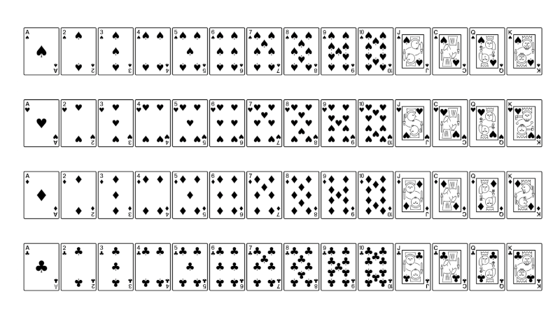
The way most people sort a hand of playing cards is a sort of greedy algorithm. They scan for the highest card and put it first. Then they scan the remainder of the hand for the next highest card and so on. This algorithm is known as insertion sort. It’s not the most efficient algorithm, but it may be the most natural, and it works. And for a hand of five cards it’s about as good as any.

Anyone who has taken an algorithms class will know you can beat insertion sort with a more sophisticated algorithm such as heap sort. But sorting is a well-understood, one-dimensional problem. That’s why people long ago came up with solutions that are better than a greedy approach. But when a problem is not well understood and is high-dimensional, greedy algorithms are more likely to succeed, even if they’re not optimal.

Training neural nets

Training a neural network is a very high dimensional optimization problem, maybe on the order of a billion dimensions. And yet it is solved using stochastic gradient descent, which is essentially a greedy algorithm. At each iteration, you move in the direction that gives you the most improvement toward your goal. There’s a little more nuance to it than that, but that’s the basic idea.

How can gradient descent work so well in practice when in theory it could get stuck in a local minimum or a saddle point? John Carmack posted a heuristic explanation on Twitter a few weeks ago. A local critical point requires the “cooperation” of every variable in the function you’re optimizing. The more variables, the less likely this is to happen.

Carmack didn’t give a full explanation—he posted a tweet, not a journal article—but he does give an intuitive idea of what’s going on. At the global minimum, the variables cooperate for a good reason. He assumes the variables are unlikely to cooperate anywhere else, which is apparently often true when training neural nets.

Usually things get harder in higher dimensions, hence the “curse of dimensionality.” But there’s a sort of blessing of dimensionality here: you’re less likely to get stuck in a local minimum in higher dimensions.

Back to the rodeo

Training a neural network can be a huge undertaking, using millions of dollars worth of electricity, but it’s a mathematically defined problem. Life goals such as becoming a rodeo clown are not cleanly quantified problems. They are very high dimensional in the sense that there are a vast number of things you could do at any given time. You might argue by analogy with neural nets that the fact that there are so many dimensions means that you’re unlikely to get stuck in a local minimum. This is a loose analogy, one that easily breaks down, but still one worth thinking about.

Seth Godin once said “Remarkable work often comes from making choices when everyone else feels as though there is no choice.” What looks like a local minimum may be revealed to not be once you consider more options.

Image by Clarence Alford from Pixabay

There’s a little program called strings that searches for what appear to be strings inside binary file. I’ll refer to it as strings(1) to distinguish the program name from the common English word strings. [1]

What does strings(1) consider to be a string? By default it is a sequence of four or more bytes that correspond to printable ASCII strings. There are command options to change the sequence length and the character encoding.

There are 98 printable ASCII characters [2] and 256 possible values for an 8-bit byte, so the probability of a byte being a printable character is

p = 98/256 = 0.3828125.

This implies that the probability of strings(1) flagging a sequence of four random bytes as a string is p⁴ or about 2%.

How long a string might you find inside a binary file?

I ran strings(1) on a photograph and found a 46-character string:

   .IEC 61966-2.1 Default RGB colour space - sRGB

Of course this isn’t random. This string is part of the metadata stored inside JPEG images.

Next I encrypted the file so that no strings would be metadata and all strings would be false positives. The longest line was 12 characters:

    Z<Bq{7fH}~G9

How does this compare to what we might expect from a random file? I wrote about the probability of long runs a dozen years ago. In a file of n bytes, the expected length of the longest run of printable characters is approximately

In my case, the file had n = 203,308 bytes. The expected length of the longest run of printable characters would then be 12.2 characters, and so the actual length of the longest run is in line with what theory would have predicted.

[1] Unix documentation is separated into sections, and parentheses after a name specify the documentation section. Section 1 is for programs, Section 2 is for system calls, etc. So, for example, chmod(1) is the command line utility named chmod, and chmod(2) is the system call by the same name. Since command line utilities often have names that are common words, tacking (1) on the end helps distinguish program names from English words.

[2] p could be a little larger if you consider some of the control characters to be printable.