Uncategorized

Typesetting Sha and Bitcoin

I went down a rabbit hole this week using two symbols in LaTeX. The first was the Russian letter Sha (Ш, U+0248), and the second was the currency symbol for Bitcoin (₿, U+20BF).

Sha

I thought there would be a LaTeX package that would include Ш as a symbol rather than as a Russian letter, just as \pi produces π as a symbol rather than as a Greek letter per se, but apparently there isn’t. I was surprised, since Ш is used in math for at least three different things [1].

When I post on @TeXtip how to produce various symbols in LaTeX, I often get a reply telling me I should simply paste in the Unicode character and use XeTeX. That’s what I ended up doing, except one does not simply use XeTeX.

You have to set the font to one that contains a glyph for the character you want, and you have to use a font encoding package. I ended up adding these two lines to my file header:

    \usepackage[T2A]{fontenc}
    \usepackage{eulervm}

That worked, but only when I compiled with pdflatex, not xelatex.

Bitcoin

I ended up using a different but analogous tactic for the Bitcoin symbol. I used fontspec, Liberation Sans, and xelatex rather than fontenc, Euler, and pdflatex. These were the lines I added to the header:

    \usepackage{fontspec}
    \setmainfont{Liberation Sans}

Without these two lines I get the error message

    Missing character: There is no ₿ (U+20BF) in font ...

I didn’t need to use ₿ and Ш in the same document, but the approach in this section works for both. The approach in the previous section will not work for ₿ because the Euler font does not contain a gylph for ₿.

Related posts

[1] The three mathematical uses of Ш that I’m aware of are the shuffle product, the Dirac comb distribution, and Tate–Shafarevich group.

Houston’s long term planning

When I hear American cities criticized for lack of long-term planning, my initial thought is that this is a good thing because the future cannot be predicted or directed very far in advance, and cities should be allowed to grow organically. Houston, in particular, is subject to a lot of criticism because of its lack of zoning, which I also think is a good thing. [1]

With that in mind, I was very surprised to see the following thread [2] from Aaron Renn.

Maybe the craziest thing about Houston’s third beltway, Grand Parkway, is that the idea originated in 1961, when the Houston metro area population was only 1.2 million people. [It’s now 7.8 million. — JC]

“In October 1965, plans for the Grand Parkway became public. The Houston City Planning Commission released a draft version of the 1966 Major Thoroughfare and Freeway Plan showing the new third loop on the official planning map.”

“The City Planning Commission approved the route and scheduled a public hearing for February 17, 1966. The Houston Chronicle enthusiastically endorsed the new route, saying, ‘No sensible citizen can doubt that this freeway will be needed eventually.’”

Aaron’s quotations are from Houston Freeways.

To a very crude approximation, a map of Houston looks like three concentric rings [2]. According to the sources cited above, planning for the outer ring began long before the middle ring was completed. The first section of the Grand Parkway opened in 1994, and it’s maybe three quarters finished currently.

Maybe what has made Houston successful is that it planned far ahead on a macro scale, but has not micromanaged as much as most cities.

[1] Along these lines, see James Scott’s book Seeing Like a State for examples of failures in long-range state planning. Or if you don’t have the to read the book, you might want to read Venkatesh Rao’s article A Big Little Idea Called Legibility.

[2] It’s not exactly a thread. It’s a series of posts that quote the first sentence.

[3] When the outer ring, the Grand Parkway, is completed, it will be the longest beltway in the US and encompass more area than the state of Rhode Island.

Another little chess puzzle

Here’s another little chess puzzle by Martin Gardner, taken from the same paper as earlier.

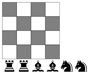
The task is to place two rooks, two bishops, and two knights on a 4 by 4 chessboard so that no piece attacks any other.

As before, there are two basic solutions, plus symmetries.

See this post for solutions, and a Prolog program that finds and enumerates the solutions.

Multiplying by quaternions on the left and right

The map that takes a quaternion x to the quaternion qx is linear, so it can be represented as multiplication by a matrix. The same is true of the map that takes x to xq, but the two matrices are not the same because quaternion multiplication does not commute.

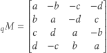
Let qa + bi + cjdk and let qM be the matrix that represents multiplication on the left by q. Then

_qM = \begin{bmatrix} a & -b & -c & -d \\ b & a & -d & c \\ c & d & a & -b \\ d & -c & b & a \\ \end{bmatrix}

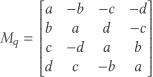
Now let Mq be the matrix that represents multiplication on the right by q. Then

M_q = \begin{bmatrix} a & -b & -c & -d \\ b & a & d & -c \\ c & -d & a & b \\ d & c & -b & a \\ \end{bmatrix}

Can prove both matrix representations are correct by showing that they do the right thing when q = 1, ij, and k. The rest follows by linearity.

You might speculate that the matrix representation for multiplying on the right by q might be the transpose of the matrix representation for multiplying on the left by q. You can look at the matrices above and see that’s not the case.

In this post I talk about how to represent rotations with quaternions, and in this post I give an equation for the equivalent rotation matrix for a rotation described by a quaternion. You can prove that the matrix representation is correct by multiplying out qM and Mq* . Keep in mind that q in that case is a unit quaterion, so the sum of the squares of its components add to 1.

Related posts

Alternative exp and log notation

The other day I stumbled on an article [1] that advocated writing ab as ab and loga(b) as ab.

\begin{align*} a &\uparrow b \equiv a^b  \\ a &\downarrow b \equiv \log_a b \end{align*}

This is a special case of Knuth’s up arrow and down arrow notation. Knuth introduces his arrows with the intention of repeating them to represent hyperexponentiation and iterated logarithms. But the emphasis in [1] is more on the pedagogical advantages of using a single up or down arrow.

Advantages

One advantage is that the notation is more symmetric. Exponents and logs are inverses of each other, and up and down arrows are visual inverses of each other.

Another advantage is that the down arrow notation makes the base of the logarithm more prominent, which is sometimes useful.

Finally, the up and down arrow notation is more typographically linear:  ab and ab stay within a line, whereas ab and loga(b) extend above and below the line. LaTeX handles subscripts and superscripts well, but HTML doesn’t. That’s one reason I usually write exp(x) rather than ex here.

Comparison

Here are the basic properties of logs and exponents using conventional notation.

\begin{align} a^b = c &\iff \log_a c = b \\ \log_b 1 &= 0 \\ \log_b b &= 1 \\ \log_b(b^x) &= x \\ b^{\log_b x} &= x \\ \log_b xy &= \log_b x + \log_b y \\ \log_b \frac{x}{y} &= \log_b x - \log_by \\ a^{\log_b c} &= c^{\log_b a} \\ \log_a b^c &= c (\log_a b) \\ (\log_b a) (\log_a x) &= \log_b x \end{align}

Here are the same properties using up and down arrow notation.

\begin{align} a \uparrow b = c &\iff a \downarrow c = b \\ b \downarrow 1 &= 0 \\ b \downarrow b &= 1 \\ b \downarrow (b \uparrow x) &= x \\ b \uparrow (b \downarrow x) &= x \\ b \downarrow xy &= b \downarrow x + b \downarrow y \\ b \downarrow \frac{x}{y} &= b \downarrow x - b \downarrow y \\ a \uparrow (b \downarrow c) &= c \uparrow (b \downarrow a ) \\ a \downarrow (b \uparrow c) &= c (a \downarrow b) \\ (b \downarrow a) (a \downarrow x) &= b \downarrow x \end{align}

Related posts

[1] Margaret Brown. Some Thoughts on the Use of Computer Symbols in Mathematics. The Mathematical Gazette, Vol. 58, No. 404 (Jun., 1974), pp. 78-79

A crowded little chess puzzle

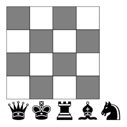
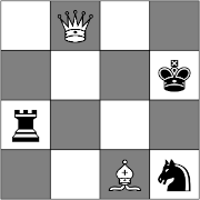
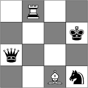
Here’s a puzzle by Martin Gardner [1].

Can a queen, king, rook, bishop, and knight be placed on a 4² board so no piece attacks another?

There are two solutions, plus symmetries.

Note that in all non-attacking chess puzzles, the colors of the pieces are irrelevant. In the solutions I chose the piece colors to be the opposite of the square colors strictly for aesthetic reasons.

More chess posts

More Martin Gardner posts

[1] Martin Gardner. Some New Results on Nonattacking Chess Tasks. Math Horizons. February 2001, pp 10–12.

The non-attacking bishops problem

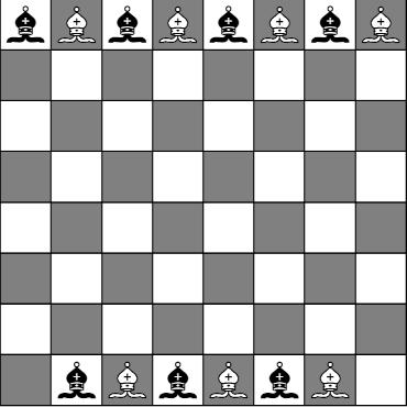
How many bishops can you place on a chessboard so that no bishop is attacking any other bishop?

For a standard 8 × 8 chessboard the answer is 14. In general, for an n × n chessboard the answer is 2n − 2.

Here’s one way to place the maximum number of non-attacking bishops.

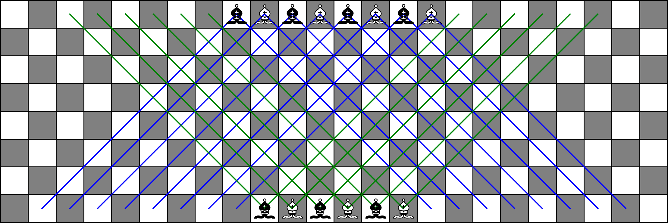
To see that the bishops cannot attack each other, I think it’s helpful to imagine extending the chessboard so that each bishop attacks the same number of squares. Then we can see that they miss each other.

Related posts

Frequency of names of English monarchs

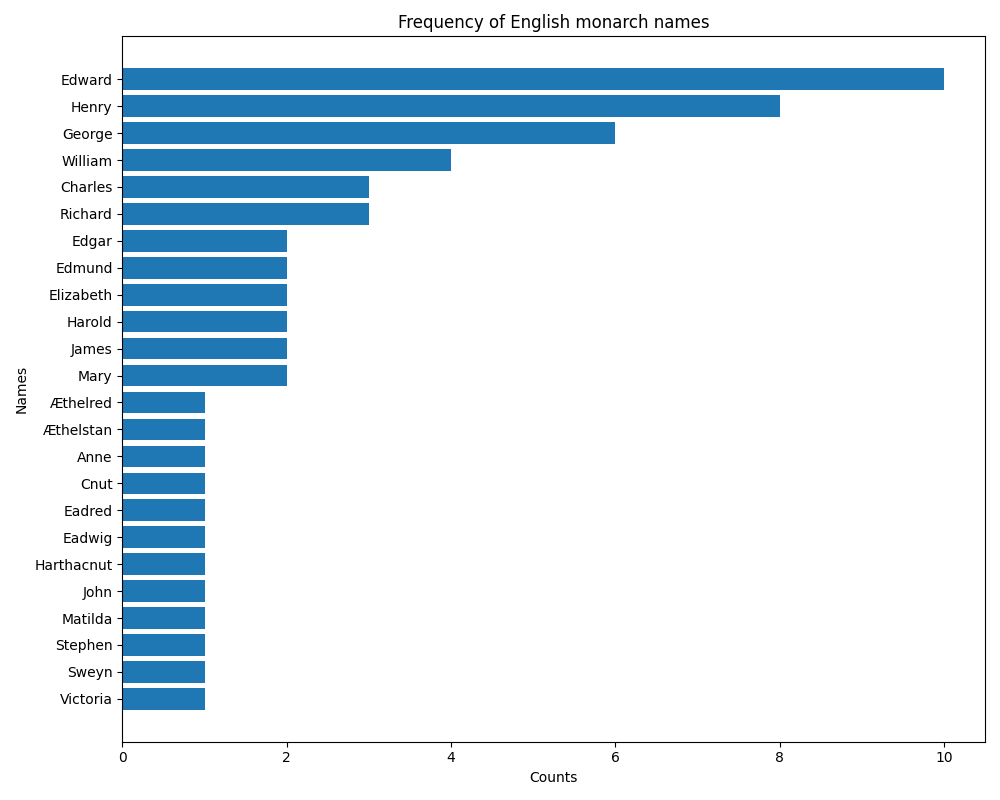
After I wrote the code to make the bar graph of papal names for the previous post, I decided to reuse the code to make a similar graph for monarchs of England. Just as there is some complication in counting papal names, there are even more complications in counting names of English monarchs.

Who was the first king of England? I went with Æthelstan (924–927). Was Lady Jane Grey queen of England? Not for my chart. Note that Edward the Elder and Edward the Martyr came before Henry I.

Incidentally, John is the most common name for a pope and the least common for a king of England. Several monarch names are unique, but John’s name is conspicuously not reused since he was an odious king. I remember my world history teacher saying there would never be another English king named John, something I found disappointing at the time.

Frequency of papal names

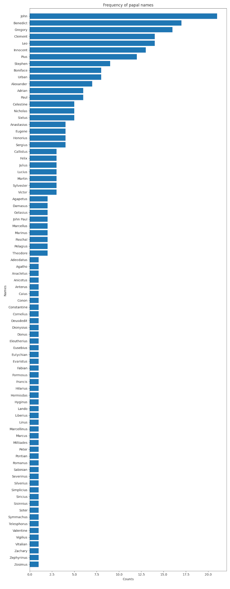
The new pope chose the name Leo XIV. That made me curious about the distribution of names of popes and so I made the graph below. (I’m Protestant, so wasn’t familiar to me.)

Looks like Leo is tied with Clement for fourth place, the top three names being John, Benedict, and Gregory.

There are a few oddities in counting the names due to the time in the Middle Ages when there was disagreement over who was pope. For this reason some popes are listed twice, sorta like how Grover Cleveland and Donald Trump each appear twice in the list of US presidents. And although the last pope named John was John XXIII, 21 popes have been named John: there was no John XX due to a clerical error, and John XVI was declared an antipope.

I also made a higher resolution PDF.

Converting between quaternions and rotation matrices

In the previous post I wrote about representing rotations with quaternions. This representation has several advantages, such as making it clear how rotations compose. Rotations are often represented as matrices, and so it’s useful to be able to go between the two representations.

A unit-length quaternion (q0, q1, q2, q3) represents a rotation by an angle θ around an axis in the direction of (q1, q2, q3) where cos(θ/2) = q0. The corresponding rotation matrix is given below.

R = \begin{pmatrix} 2(q_0^2 + q_1^2) - 1 & 2(q_1 q_2 - q_0 q_3) & 2(q_1 q_3 + q_0 q_2) \\ 2(q_1 q_2 + q_0 q_3) & 2(q_0^2 + q_2^2) - 1 & 2(q_1 q_3 - q_0 q_1) \\ 2(q_1 q_3 - q_0 q_2) & 2(q_2 q_3 + q_0 q_1) & 2(q_0^2 + q_3^2) - 1 \end{pmatrix}

(Update: there was a typo in the equation above. See this post for how Claude found the typo and wrote Lean code to verify the fix.)

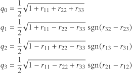
Going the other way around, inferring a quaternion representation from a rotation matrix, is harder. Here is a mathematically correct but numerically suboptimal method known [1] as the Chiaverini-Siciliano method.
\begin{align*} q_0 &= \frac{1}{2} \sqrt{1 + r_{11} + r_{22} + r_{33}} \\ q_1 &= \frac{1}{2} \sqrt{1 + r_{11} - r_{22} - r_{33}} \text{ sgn}(r_{32} - r_{23}) \\ q_2 &= \frac{1}{2} \sqrt{1 - r_{11} + r_{22} - r_{33}} \text{ sgn}(r_{13} - r_{31}) \\ q_3 &= \frac{1}{2} \sqrt{1 - r_{11} - r_{22} + r_{33}} \text{ sgn}(r_{21} - r_{12}) \end{align*}

Here sgn is the sign function; sgn(x) equals 1 if x is positive and −1 if x is negative. Note that the components only depend on the diagonal of the rotation matrix, aside from the sign terms. Better numerical algorithms make more use of the off-diagonal elements.

Accounting for degrees of freedom

Something seems a little suspicious here. Quaternions contain four real numbers, and 3 by 3 matrices contain nine. How can four numbers determine nine numbers? And going the other way, out of the nine, we essentially choose three that determine the four components of a quaternion.

Quaternions have four degrees of freedom, but we’re using unit quaternions, so there are basically three degrees of freedom. Likewise orthogonal matrices have three degrees of freedom. An axis of rotation is a point on a sphere, so that has two degrees of freedom, and the degree of rotation is the third degree of freedom.

In topological terms, the unit quaternions and the set of 3 by 3 orthogonal matrices are both three dimensional manifolds, and the former is a double cover of the latter. It is a double cover because a unit quaternion q corresponds to the same rotation as −q.

Python code

Implementing the equations above is straightforward.

import numpy as np

def quaternion_to_rotation_matrix(q):
    q0, q1, q2, q3 = q
    return np.array([
        [2*(q0**2 + q1**2) - 1, 2*(q1*q2 - q0*q3), 2*(q1*q3 + q0*q2)],
        [2*(q1*q2 + q0*q3), 2*(q0**2 + q2**2) - 1, 2*(q2*q3 - q0*q1)],
        [2*(q1*q3 - q0*q2), 2*(q2*q3 + q0*q1), 2*(q0**2 + q3**2) - 1]
    ]) 

def rotation_matrix_to_quaternion(R):
    r11, r12, r13 = R[0, 0], R[0, 1], R[0, 2]
    r21, r22, r23 = R[1, 0], R[1, 1], R[1, 2]
    r31, r32, r33 = R[2, 0], R[2, 1], R[2, 2]
    
    # Calculate quaternion components
    q0 = 0.5 * np.sqrt(1 + r11 + r22 + r33)
    q1 = 0.5 * np.sqrt(1 + r11 - r22 - r33) * np.sign(r32 - r23)
    q2 = 0.5 * np.sqrt(1 - r11 + r22 - r33) * np.sign(r13 - r31)
    q3 = 0.5 * np.sqrt(1 - r11 - r22 + r33) * np.sign(r21 - r12)
    
    return np.array([q0, q1, q2, q3])

Random testing

We’d like to test the code above by generating random quaternions, converting the quaternions to rotation matrices, then back to quaternions to verify that the round trip puts us back essentially where we started. Then we’d like to go the other way around, starting with randomly generated rotation matrices.

To generate a random unit quaternion, we generate a vector of four independent normal random values, then normalize by dividing by its length. (See this recent post.)

To generate a random rotation matrix, we use a generator that is part of SciPy.

Here’s the test code:

def randomq():
    q = norm.rvs(size=4)
    return q/np.linalg.norm(q)

def randomR():
    return special_ortho_group.rvs(dim=3)

np.random.seed(20250507)
N = 10

for _ in range(N):
    q = randomq()
    R = quaternion_to_rotation_matrix(q)
    t = rotation_matrix_to_quaternion(R)
    print(np.linalg.norm(q - t))
    
for _ in range(N):
    R = randomR()
    q = rotation_matrix_to_quaternion(R)
    T = quaternion_to_rotation_matrix(q)
    print(np.linalg.norm(R - T))

The first test utterly fails, returning six 2s, i.e. the round trip vector is as far as possible from the vector we started with. How could that happen? It must be returning the negative of the original vector. Now go back to the discussion above about double covers: q and −q correspond to the same rotation.

If we go back and add the line

    q *= np.sign(q[0])

then we standardize our random vectors to have a positive first component, just like the vectors returned by rotation_matrix_to_quaternion.

Now our tests all return norms on the order of 10−16 to 10−14. There’s a little room to improve the accuracy, but the results are good.

Update: I did some more random testing, and found errors on the order of 10−10. Then I was able to create a test case where rotation_matrix_to_quaternion threw an exception because one of the square roots had a negative argument. In [1] the authors get around this problem by evaluating two theoretically equivalent expressions for each of the square root arguments. The expressions are complementary in the sense that both should not lead to numerical difficulties at the same time.

[1] See “Accurate Computation of Quaternions from Rotation Matrices” by Soheil Sarabandi and Federico Thomas for a better numerical algorithm. See also the article “A Survey on the Computation of Quaternions From Rotation Matrices” by the same authors.