Partition symmetry

Posted on 16 November 2021 by John

Let p(M, N, n) be the number of partitions of the integer n into at most M parts, each containing integers at most N. Then

p(M, N, n) = p(N, M, n).

That is, you can swap the size of the partition multisets and the upper bound on the elements in the multisets.

For example, lets look at the partitions of 6 into multisets with at most 3 elements. The Mathematica command

    IntegerPartitions[6, 3]

returns

{6}
{5, 1}
{4, 2}
{4, 1, 1}
{3, 3}
{3, 2, 1}
{2, 2, 2}

Now let’s look at the partitions of 6 into sets with any number of elements, but with no elements greater than 3. The Mathematica command

    IntegerPartitions[6, All, {1, 2, 3}]

returns

{3, 3}
{3, 2, 1}
{3, 1, 1, 1}
{2, 2, 2}
{2, 2, 1, 1}
{2, 1, 1, 1, 1}
{1, 1, 1, 1, 1, 1}}

Both return a list of 7 multisets because

p(3, 6, 6) = p(6, 3, 6) = 7.

As another example, let’s look at partitions of 11. First we look at partitions with at most 3 elements, with each element less than or equal to 5. We list these with

    IntegerPartitions[11, 3, Range[5]]

which gives

{5, 5, 1}
{5, 4, 2}
{5, 3, 3}
{4, 4, 3}

Now let’s look at partitions of 11 into multisets with at most 5 elements, each less than or equal to 3 using

    IntegerPartitions[11, 5,  Range[3]]

This gives us

{5, 5, 1}
{5, 4, 2}
{5, 3, 3}
{4, 4, 3}

Not only do both lists have the same number of partitions, which we would expect because

p(3, 5, 11) = p(5, 3, 11),

in this case they actually give the same list of partitions.

The symmetry relation here follows from the symmetry of the q-binomial coefficient because p(M, N, n) equals the coefficient of qⁿ in the q-binomial

$\binom{M+N}{N}_q = \binom{M+N}{M}_q$

It’s not immediately obvious from the definition that the rational function defining q-binomial coefficient is in fact a polynomial, but it is.

Estimating the number of integer partitions

Posted on 14 November 2021 by John

Last week I wrote a few posts that included code that iterated over all partitions of a positive integer n. See here, here, and here. How long would it take these programs to run for large n?

For this post, I’ll focus just on how many partitions there are. It’s interesting to think about how you would generate the partitions, but that’s a topic for another time.

Ramanujan discovered an asymptotic formula for p(n), the number of partitions of n. As n increases,

$p(n) \sim \frac{1}{4n\sqrt{3}} \exp\left( \pi \sqrt{\frac{2n}{3}} \right)$

The ratio of the two sides of the equation goes to 1 as n → ∞, but how accurate is it for the sizes of n that you might want to iterate over in a program?

Before answering that, we need to decide what range of n we might use. Let’s be generous and say we might want to look at up to a trillion (10¹²) partitions. How big of a value of n does that correspond to? The estimate above shows p(200) is on the order of 4 × 10¹², so we only need to be concerned with n ≤ 200. (See the next post for how to exactly solve for a n that gives a specified value.)

Here’s a plot to show the relative error in the approximation above.

Here’s the Mathematica code that made the plot.

    approx[n_] := Exp[Pi Sqrt[2 n/3]]/(4 n Sqrt[3])
    DiscretePlot[ 1 - approx[n]/PartitionsP[n], {n, 200}]

So the estimate above is always an under-estimate, at least about 4% low over the range we care about. It’s good enough for a quick calculation. It tells us, for example, to be very patient if we’re going to run any program that needs to iterate over all partitions of an integer even as small as 100.

The function PartitionsP above returns the number of partitions in its argument. It returned quickly, so it certainly did not generate all partitions and count them. Algorithms for computing p(n) might make an interesting blog post another time.

Even though it would be impractical to iterate over the partitions of larger values, we still might be curious what the plot above looks like for larger arguments. Let’s see what the plot would look like for n between 200 and 2000.

The shape of the curve is practically the same.

The relative error dropped by about a factor or 3 when we increased n by a factor of 10. So we’d expect if we increase n by another factor of 10, the relative error would drop about another factor of 3, and indeed that’s what happens: when n = 20,000, the relative error is about -0.003.

Another pentagonal number theorem

Posted on 11 November 2021 by John

An earlier post presented Euler’s pentagonal number theorem. This post presents a similar theorem by N. J. Fine developed two centuries later.

Define the jth pentagonal number by

P_j = j(3j – 1) / 2

where j can be any integer, e.g. j can be negative.

Theme

Let D_e(n) is the number of distinct partitions of n of even length and D_o(n) is the number distinct partitions of odd length. (See this post if any of these terms are unfamiliar.)

Euler’s pentagonal number theorem says

$D_e(n) - D_o(n) = \left\{ \begin{array}{ll} (-1)^j & \mbox{if } n = P_j \\ 0 & \mbox{otherwise} \end{array} \right.$

Variation

Euler discovered his theorem in 1741 and proved it a few years later. N. J. Fine published [1] the following variation on Euler’s theorem in 1948.

Define π_e(n) to be the number of partitions of n into distinct numbers, the largest of which is even, and define π_o(n) to be the number of partitions of n into distinct numbers, the largest of which is odd. Then Fine’s theorem says

$\pi_e(n) - \pi_o(n) = \left\{ \begin{array}{ll} -1 & \mbox{if } n = P_j \mbox{ for } j > 0 \\ \phantom{-}1 & \mbox{if } n = P_j \mbox{ for } j < 0 \\ \phantom{-}0 & \mbox{otherwise} \end{array} \right.$

Note that Euler and Fine have different ways of defining parity, the length of a partition versus the parity of the largest element. So, for example,

{8, 3, 2}

would count as an odd partition of 13 for Euler’s theorem, because it has length 3, but an even partition for Fine’s theorem, because the largest element is 8.

Both produce ±1 for pentagonal numbers and 0 otherwise. But the sign in Euler’s theorem depends on the parity of the index j. The parity in Fine’s theorem depends on the sign of j.

Mathematica

As in the previous two posts, we will illustrate the theorem here with Mathematica.

    distinctPartitionQ[list_] := Length[list] == Length[Union[list]]

    check[n_] := 
        Total[Map[(-1)^Max[#] &, 
              Select[IntegerPartitions[n], distinctPartitionQ]]] 

    Table[{n, check[n]}, {n, 1, 8}]

This returns

    {{1, -1}, {2, 1}, {3, 0}, {4, 0}, 
     {5, -1}, {6, 0}, {7, 1}, {8, 0}}

We get -1 for n = 1 = P₁ and for n = 5 = P₂.

We get 1 for n = 2 = P_-1 and for n = 7 = P_-2.

We get 0 for all other inputs because they are not pentagonal numbers.

[1] I found this in “Euler’s Pentagonal Number Theorem” by George E. Andrews, Mathematics Magazine, Vol. 56, No. 5 (Nov., 1983), pp. 279-284. Andrews cites “Some new results on partitions” by N. J. Fine, Proc. Nat. Acad. Sci. U.S.A., 34 (1948) 616-618.

Odd parts and distinct parts

Posted on 11 November 2021 by John

The previous post looked at a result of Euler regarding even and odd distinct partitions. This post will illustrate a related theorem by Euler.

Definitions

A partition of a positive integer n is a way of writing n as the sum of positive integers, without distinguishing the order of the terms, only the multi-set of summands.

For example, 6 can be written as

1 + 2 + 3

or as

3 + 2 + 1,

but these count as the same partition. Another possible partition of 6 is

3 + 1 + 1 + 1.

Here the summands form a multistet

{3, 1, 1, 1}.

This is not a set because the 1’s appear more than once. If the multiset of summands is actually a set, the partition is called a distinct partition.

A partition is called odd if every element is odd, and even if every element is even.

Theorem

Now we can state Euler’s theorem: The number of odd partitions of an integer equals the number of distinct partitions.

As before we will illustrate this with Mathematica.

Mathematica

First we define a couple predicate functions.

    distinctPartitionQ[list_] := Length[list] == Length[Union[list]]
    oddPartitionQ[list_] := And @@ Map[OddQ, list]

There are six odd partitions of 8:

    In: Select[IntegerPartitions[8], oddPartitionQ]
    Out: {{7, 1}, {5, 3}, {5, 1, 1, 1}, {3, 3, 1, 1}, 
          {3, 1, 1, 1, 1, 1}, {1, 1, 1, 1, 1, 1, 1, 1}}

And six distinct partitions of 8:

    In: Select[IntegerPartitions[8], distinctPartitionQ]
    Out: {{8}, {7, 1}, {6, 2}, {5, 3}, {5, 2, 1}, {4, 3, 1}}

To try partitions of more numbers, let’s define

    d[n_] := Length[Select[IntegerPartitions[n], distinctPartitionQ]] - 
             Length[Select[IntegerPartitions[n], oddPartitionQ]]

We can see that d[n] is 0 for n = 1, 2, 3, …, 50 by running

    Table[d[n], {n, 1, 50}]

Testing understanding

This post and the previous post illustrate something important: it helps to verify a theorem computationally, even if you know the theorem is true, in order to test your understanding of the theorem. If a theorem by Euler were wrong, we’d know by now. But my interpretation of the terms in this theorem and the theorem in the previous post were both wrong at first, and computations made this obvious.

Note that in this post, “odd partition” means a partition consisting of only odd numbers.

In the previous post, an “odd distinct partition” is a distinct partition of odd length. If we defined “odd distinct partition” to be a distinct partition consisting of only odd numbers, the statement of Euler’s pentagonal number theorem would be false.

For example, consider the distinct partitions of 3: 3 and 2+1. One distinct partition of even length and one of odd length, as the pentagonal number theorem predicts. But of these two partitions, one consists entirely of odd numbers, and none consists entirely of even numbers.

Partitions and Pentagons

Posted on 10 November 2021 by John

This post will present a remarkable theorem of Euler which makes a connection between integer partitions and pentagons.

Partitions

A partition of an integer n is a way of writing n as a sum of positive integers. For example, there are seven unordered partitions of 5:

5
4 + 1
3 + 2
3 + 1 + 1
2 + 2 + 1
2 + 1 + 1 + 1
1 + 1 + 1 + 1 + 1

Note that order does not matter. For instance, 4 + 1 and 1 + 4 count as the same partition. You can get a list of partitions of n in Mathematica with the function IntegerPartitions[n]. If we enter IntegerPartitions[5] we get

     {{5}, {4, 1}, {3, 2}, {3, 1, 1}, {2, 2, 1}, 
      {2, 1, 1, 1}, {1, 1, 1, 1, 1}}

We say a partition is distinct if all the numbers in the sum are distinct. For example, these partitions of 5 are distinct

5
4 + 1
3 + 2

but these are not

3 + 1 + 1
2 + 2 + 1
2 + 1 + 1 + 1
1 + 1 + 1 + 1 + 1

because each has a repeated number.

We can divide distinct partitions into those having an even number of terms and those having an odd number of terms. In the example above, there is one odd partition, just 5, and two even partitions: 4 + 1 and 3 + 2.

Pentagonal numbers

The pentagonal numbers are defined by counting the number of dots in a graph of concentric pentagons: 1, 5, 12, 22, …. This is OEIS sequence A000326.

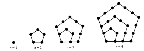
The jth pentagonal number is

P_j = j(3j – 1) / 2.

We can define negative pentagonal numbers by plugging negative values of j into the equation above, though these numbers don’t have the same geometric interpretation. (I think they do have a geometric interpretation, but I forget what it is.)

Euler’s pentagonal number theorem

Leonard Euler discovered that the number of even distinct partitions of n equals the number of odd distinct partitions, unless n is a pentagonal number (including negative indices). If n is the jth pentagonal number, then the difference between the number of even and odd distinct partitions of n equals (-1)^j. In symbols,

$D_e(n) - D_o(n) = \left\{ \begin{array}{ll} (-1)^j & \mbox{if } n = P_j \\ 0 & \mbox{otherwise} \end{array} \right.$

Here D_e is the number of even distinct partitions and D_o is the number of odd distinct partitions.

Euler discovered this by playing around with power series and noticing that the series involved were generating functions for pentagonal numbers. Jordan Bell has written a commentary on Euler’s work and posted it on arXiv.

Mathematica examples

Let’s look at the partitions of 12, the 3rd pentagonal number.

IntegerPartions[12] shows there are 77 partitions of 12. We can pick out just the partitions into distinct numbers by selecting partition sets that have no repeated terms, i.e. that have as many elements as their union.

    Select[IntegerPartitions[12], Length[Union[#]] == Length[#] &]

This returns a list of 15 partitions:

    {{12},      {11, 1},   {10, 2},      {9, 3},    {9, 2, 1}, 
     {8, 4},    {8, 3, 1}, {7, 5},       {7, 4, 1}, {7, 3, 2}, 
     {6, 5, 1}, {6, 4, 2}, {6, 3, 2, 1}, {5, 4, 3}, {5, 4, 2, 1}}

Of these sets, 7 have an even number of elements and 8 have an odd number of elements. This matches what Euler said we would get because

7 – 8 = (-1)³.

We’d like to eplore this further without having to count partitions by hand, so let’s define a helper function.

    f[list_] := Module[
        {n = Length[Union[list]]}, 
        If [n == Length[list], (-1)^n, 0]
    ]

This function returns 0 for lists that have repeated elements. For sets with no repeated elements, it returns 1 for sets with an even number of elements and -1 for sets with an odd number of elements. If we apply this function to the list of partitions of n and take the sum, we get

D_e(n) – D_o(n).

Now

    Total[Map[f, IntegerPartitions[12]]]

returns -1. And we can verify that it returns (-1)^j for the jth pentagonal number. The code

    Table[Total[Map[f, IntegerPartitions[j (3 j - 1)/2]]], {j, -3, 3}]

returns

    {-1, 1, -1, 1, -1, 1, -1}

We can compute D_e(n) – D_o(n) for n = 1, 2, 3, …, 12 with

    Table[{n, Total[Map[f, IntegerPartitions[n]]]}, {n, 1, 12}]

and get

    {{1, -1}, {2, -1}, {3,  0}, {4,  0}, 
     {5,  1}, {6,  0}, {7,  1}, {8,  0}, 
     {9,  0}, {10, 0}, {11, 0}, {12, -1}}

which shows that we get 0 unless n is a pentagonal number.

Euler characteristic

Euler’s pentagonal number theorem reminds me of Euler characteristic. Maybe there’s a historical connection there, or maybe someone could formalize a connection even if Euler didn’t make the connection himself. In its most familiar form, the Euler characteristic of a polyhedron is

V – E + F

where V is the number of vertices, E is the number of edges, and F is the number of faces. Notice that this is an alternating sum counting o-dimensional things (vertices), 1-dimensional things (edges), and 2-dimensional things (faces). This is extended to higher dimensions, defining the Euler characteristic to be the alternating sum of dimensions of homology groups.

We can write D_e(n) – D_o(n) to make it look more like the Euler characteristic, using D_k(n) to denote the number of distinct partitions of size k.

D₀(n) – D₁(n) + D₂(n) – …

I suppose there’s some way to formulate Euler’s pentagonal number theorem in terms of homology.

Partitions

Partition symmetry

More partition posts

Estimating the number of integer partitions

Another pentagonal number theorem

Theme

Variation

Mathematica

Related

Odd parts and distinct parts

Definitions

Theorem

Mathematica

Testing understanding

Partitions and Pentagons

Partitions

Pentagonal numbers

Euler’s pentagonal number theorem

Mathematica examples

Euler characteristic