Comparing two ways to fit a line to data

Suppose you have a set of points and you want to fit a straight line to the data. I’ll present two ways of doing this, one that works better numerically than the other.

Given points (x₁, y₁), …, (x_N, y_N) we want to fit the best line of the form y = mx + b, best in the sense of minimizing the square of the differences between the actual data y_i values and the predicted values mx_i + b.

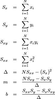
The textbook solution is the following sequence of equations.

The equations above are absolutely correct, but turning them directly into software isn’t the best approach. Given vectors of x and y values, here is C++ code to compute the slope m and the intercept b directly from the equations above.

	double sx = 0.0, sy = 0.0, sxx = 0.0, sxy = 0.0;
	int n = x.size();
	for (int i = 0; i < n; ++i)
	{
		sx += x[i];
		sy += y[i];
		sxx += x[i]*x[i];
		sxy += x[i]*y[i];
	}
	double delta = n*sxx - sx*sx;
	double slope = (n*sxy - sx*sy)/delta;
	double intercept = (sxx*sy - sx*sxy)/delta;

This direct method often works. However, it presents multiple opportunities for loss of precision. First of all, the Δ term is the same calculation criticized in this post on computing standard deviation. If the x values are large relative to their variance, the Δ term can be inaccurate, possibly wildly inaccurate.

The problem with computing Δ directly is that it could potentially require subtracting nearly equal numbers. You always want to avoid computing a small number as the difference of two big numbers if you can. The equations for slope and intercept have a similar vulnerability.

The second method is algebraically equivalent to the method above, but it is better suited to numerical calculation. Here it is in code.

	double sx = 0.0, sy = 0.0, stt = 0.0, sts = 0.0;
	int n = x.size();
	for (int i = 0; i < n; ++i)
	{
		sx += x[i];
		sy += y[i];
	}
	for (int i = 0; i < n; ++i)
	{
		double t = x[i] - sx/n;
		stt += t*t;
		sts += t*y[i];
	}

	double slope = sts/stt;
	double intercept = (sy - sx*slope)/n;

This method involves subtraction, and it too can fail for some data sets. But in general it does better than the former method.

Here are a couple examples to show how the latter method can succeed when the former method fails.

First we populate x and y as follows.

	for (int i = 0; i < numSamples; ++i)
	{
		x[i] = 1e10 + i;
		y[i] = 3*x[i] + 1e10 + 100*GetNormal();
	}

Here GetNormal() is generator for standard normal random variables. Aside from some small change due to the random noise, we would expect slope 3 and intercept 10¹⁰.

The most direct method gives slope -0.666667 and intercept 5.15396e+10. The better method gives slope: 3.01055 and intercept: 9.8945e+9. If we remove the Gaussian noise and try again, the direct method gives slope 3.33333 and intercept 5.72662e+9 while the better method is exactly correct: slope 3 intercept and 1e+10.

As another example, fill x and y as follows.

	for (int i = 0; i < numSamples; ++i)
	{
		x[i] = 1e6*i;
		y[i] = 1e6*x[i] + 50 + GetNormal();
	}

Now both method compute the intercept exactly as 1e6 but the direct method computes the intercept as 60.0686 while the second method computes 52.416. Neither is very close to the theoretical value of 50, but the latter method is closer.

To read more about why one way can be so much better than the other, see this writeup on the analogous issue with computing standard deviation: theoretical explanation for numerical results.

Update: See related post on computing correlation coefficients.

Related: Linear regression is more than curve-fitting