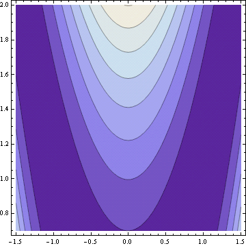
Rosenbrock’s banana function is a famous test case for optimization software. It’s called the banana function because of its curved contours.
The definition of the function is

The function has a global minimum at (1, 1). If an optimization method starts at the point (−1.2, 1), it has to find its way to the other side of a flat, curved valley to find the optimal point.
Rosenbrock’s banana function is just one of the canonical test functions in the paper “Testing Unconstrained Optimization Software” by Moré, Garbow, and Hillstrom in ACM Transactions on Mathematical Software Vol. 7, No. 1, March 1981, pp 17-41. The starting point (−1.2, 1) mentioned above comes from the starting point required in that paper.
I mentioned a while back that I was trying out Python alternatives for tasks I have done in Mathematica. I tried making contour plots with Python using matplotlib. This was challenging to figure out. The plots did not look very good, though I imagine I could have made satisfactory plots if I had explored the options. Instead, I fired up Mathematica and produced the plot above easily using the following code.
Banana[x_, y_] := (1 - x)^2 + 100 (y - x*x)^2
ContourPlot[Banana[x, y], {x, -1.5, 1.5}, {y, 0.7, 2.0}]
John, don’t give up on Python! In SAGE, that will be something like
x,y = var(‘x,y’)
banana(x,y) = (1 – x)^2 + 100*(y – x*x)^2
contour_plot(banana(x,y),(x,-1.5, 1.5), (y, 0.7, 2.0),cmap=’pink’)
And in matplotlib it’s something like
from pylab import mgrid, contourf, cm, show

f = lambda x,y: (1 - x)**2 + 100*(y - x**2)**2

x,y = mgrid[-1.5:1.5:50j, 0.7:2:50j]

contourf(x, y, f(x,y), cmap=cm.Purples_r)

show()
+1 for Sage, and it’s even easier than Sergey makes it look; since variables get automatically recognized in a function definition, you can skip the line
x, y = var('x,y')
and go straight to
banana(x, y) = (1 - x)^2 + 100(y - x * x)^2
The “cmap” option in contour_plot is optional as well.
Sorry to post again, but Sage also handles the optimization question nicely; using the “minimize” command, which can use a couple of different algorithms to find the minimum of a function:
sage: minimize(banana, [-1.2, 1], algorithm='powell')

Optimization terminated successfully.

Current function value: 0.000000

Iterations: 23

Function evaluations: 665

(1.0, 1.0)
If I had left the “algorithm” option blank, I think it would have used Broyden-Fletcher-Goldfarb-Shannon. This algorithm yielded a slightly different answer.
Hi John.
Jon Harrop (Flying Frog) wrote about gradient and used banana to illustrate; no plot though.
http://fsharpnews.blogspot.com/2011/01/gradient-descent.html
And the following defines the famous Rosenbrock “banana” function that is notoriously difficult to minimize due to its curvature around the minimum:
> let rosenbrock (xs: vector) =
let x, y = xs.[0], xs.[1]
pown (1.0 – x) 2 + 100.0 * pown (y – pown x 2) 2;;
val rosenbrock : vector -> floatThe minimum at (1, 1) may be found quickly and easily using the functions defined above as follows:
> let xs =
vector[0.0; 0.0]
|> gradientDescent rosenbrock (grad rosenbrock);;
val xs : Vector = vector [|0.9977180571; 0.99543389|]
Has anyone plotted 2d cross sections of the 4d or 10d http://en.wikipedia.org/wiki/Rosenbrock_function ?
There is a very simple algorithm that is competitive with current genetic and ES algorithms.
I have some example code here:
http://www.mediafire.com/?8i1pjhesw6s4oj7
Well it is an ES algorithm but it uses a multi-scale approach. It is similar to Continuous Gray Code optimization. A few other people have come up with basically the same idea in the past.
I also have some code on the Walsh Hadamard transform you may peruse if you wish:
http://www.mediafire.com/?q4o3clxu1r18ufs
But I have to say that some ideas in that are only joyful playing.