Lagrange multiplier setup: Now what?

Suppose you need to optimize, i.e. maximize or minimize, a function f(x). If this is a practical problem and not a textbook exercise, you probably need to optimize f(x) subject to some constraint on x, say g(x) = 0.

Hmm. Optimize one function subject to a constraint given by another function. Oh yeah, Lagrange multipliers! You just need to solve

\nabla f = \nabla g

Or maybe you have two constraints: g(x) = 0 and h(x) = 0. No big deal. Just introduce another Lagrange multiplier:

\nabla f = \lambda_1 \nabla g + \lambda_2 \nabla h

OK. Now what?

Suppose your x is an n-dimensional vector, and you have k constraints. Now you have a system of n + k equations in n + k unknowns, one equation for each component of the Lagrange multiplier equation and one equation for each constraint.

If your system of equations is linear, hurrah! Maybe it won’t be hard to find where your function takes on its maximum and minimum values [1].

But in general you have a system of nonlinear equations, potentially a lot of nonlinear equations in a lot of unknowns. Maybe you’re new problem is harder than your original problem. That is, it might be easier to optimize your original function, subject to its constraints, using a different method than to solve the nonlinear system of equations that applying Lagrange multipliers gives you.

How do you solve a system of nonlinear equations? That’s a hard question because “nonlinear” is not a hypothesis; it’s the negation of a hypothesis. Suppose I tell you I’m thinking of an animal, and it’s not an elephant. That’s not much to go on. Non-linear is sorta like non-elephantine: you’ve said what a thing is not, but you haven’t said what it is.

One way for functions to be nonlinear is to be convex; convexity is often a tractable generalization of linearity. If your original optimization problem is convex, i.e. both the objective function and the constraints are convex functions, then directly solving your optimization problem may be easier than introducing Lagrange multipliers.

Another class of nonlinear functions is polynomials. If Lagrange multipliers give you a system of several polynomial equations in several unknowns, you may be able to solve your system of equations using techniques from algebraic geometry.

If your equations do not involve polynomial functions, but do involve functions that can be adequately approximated by polynomial functions, maybe the algebraic geometry route will work. But “adequate” here means that the solution to the approximate problem, the polynomial problem, gives a sufficiently accurate solution to the original problem. That may be hard to assess.

Your initial exposure to Lagrange multipliers in a calculus class may have left the wrong impression. Calculus textbooks are filled carefully contrived exercises that can be solved in a moderate amount of time, and for good reason. The problems you solve for exercises are not intrinsically important; you’re solving them to learn a technique. But in a real application, where the problem is intrinsically important (and the solution technique is not) things might be a lot harder.

Related posts

[1] If then system of equations is linear, then your optimization problem must have a very special form: optimizing a quadratic objective function subject to linear constraints, i.e. a quadratic programming problem.

Best approximation of a catenary by a parabola

A parabola and a catenary can look very similar but are not the same. The graph of

y = x²

is a parabola and the graph of

y = cosh(x) = (ex + ex)/2

is a catenary. You’ve probably seen parabolas in a math class; you’ve seen a catenary if you’ve seen the St. Louis arch.

Depending on the range and scale, parabolas and catenaries can be too similar to distinguish visually, though over a wide range enough range the exponential growth of the catenary becomes apparent.

For example, for x between -1 and 1, it’s possible to scale a parabola to match a catenary so well that the graphs practically overlap. The blue curve is a catenary and the orange curve is a parabola.

The graph above looks orange because the latter essentially overwrites the former. The relative error in approximating the catenary by the parabola is about 0.6%.

But when x ranges over -10 to 10, the best parabola fit is not good at all. The catenary is much flatter in the middle and much steeper in the sides. On this wider scale the hyperbolic cosine function is essentially e|x|.

Here’s an intermediate case, -3 < x < 3, where the parabola fits the catenary pretty well, though one can easily see that the curves are not the same.

Now for some details. How are we defining “best” when we say best fit, and how do we calculate the parameters for this fit?

I’m using a least-squares fit, minimizing the L² norm of the error, over the interval [M, M]. That is, I’m approximating

cosh(x)

with

c + kx²

and finding c and k that minimize the integral

\int_{-M}^M (\cosh(x) - c - kx^2)^2\, dx

The optimal values of c and k vary with M. As M increases, c decreases and k increases.

It works out that the optimal value of c is

-\frac{3 \left(M^2 \sinh (M)+5 \sinh (M)-5 M \cosh (M)\right)}{2 M^3}

and the optimal value of k is

\frac{15 \left(M^2 \sinh (M)+3 \sinh (M)-3 M \cosh (M)\right)}{2 M^5}

Here’s a log-scale plot of the L² norm of the error, the square root of the integral above, for the optimal parameters as a function of M.

More on catenaries

Inverse optimization

This morning Patrick Honner posted the image below on Twitter.

The image was created by Robert Bosch by solving a “traveling salesman” problem, finding a nearly optimal route for passing through 12,000 points.

I find this interesting for a couple reasons. For one thing, I remember when the traveling salesman problem was considered intractable. And in theory it still is! But in practice it is not difficult now to find nearly optimal solutions for very large traveling salesman problems.

Another reason I find this interesting is that there is a higher-level problem in the background, the problem of constructing a problem whose solution gives you a desired image.

Robert Bosch is showing us a solution to two problems. The image above is the solution to an optimization problem, and the problem it solves is itself the solution to another problem in the background. He’s doing a sort of inverse optimization, searching for an optimization problem. He goes into some of his techniques in his recent book Opt Art which I wrote about here.

This gets back to an argument I’ve had with statisticians who are resistant to innovative methods. They’ll say “But our method is optimal. You can’t do any better by definition. End of discussion!” But every method is optimal by some criteria. The question is whether the method is optimal by criteria appropriate to the problem at had or whether it is only optimal according to criteria that were mathematically convenient at the time it was formulated.

Robert Bosch has shown beautifully that any image can be viewed as the solution to an optimization problem. Of course the problem has to be crafted for the image. If he were solving a naturally occurring problem, such as planning a tour for an actual sales rep, and the solution had an uncanny resemblance to a piece of art by Michelangelo, that would be astounding.

More optimization posts

ADFGVX cipher and Morse code separation

A century ago the German army used a field cipher that transmitted messages using only six letters: A, D, F, G, V, and X. These letters were chosen because their Morse code representations were distinct, thus reducing transmission error.

The ADFGVX cipher was an extension of an earlier ADFGV cipher. The ADFGV cipher was based on a 5 by 5 grid of letters. The ADFGVX extended the method to a 6 by 6 grid of letters and digits. A message was first encoded using the grid coordinates of the letters, then a transposition cipher was applied to the sequence of coordinates.

This post revisits the design of the ADFGVX cipher. Not the encryption method itself, but the choice of letters used for transmission. How would you quantify the difference between two Morse code characters? Given that method of quantification, how good was the choice of ADFGV or its extension ADFGVX? Could the Germans have done better?

Quantifying separation

There are several possible ways to quantify how distinct two Morse code signals are.

Time signal difference

My first thought was to compare the signals as a function of time.

There are differing conventions for how long a dot or dash should be, and how long the space between dots and dashes should be. For this post, I will assume a dot is one unit of time, a dash is three units of time, and the space between dots or dashes is one unit of time.

The letter A is represented by a dot followed by a dash. I’ll represent this as 10111: on for one unit of time for the dot, off for one unit of time for the space between the dot and the dash, and on for three units of time for the dash. D is dash dot dot, so that would be 1110101.

We could quantify the difference between two letters in Morse code as the Hamming distance between their representations as 0s and 1s, i.e. the number of positions in which the two letters differ. To compare A and D, for example, I’ll pad the A with a couple zeros on the end to make it the same length as D.

    A: 1011100
    D: 1110101
        x x  x

The distance is 3 because the two sequences differ in three positions. (Looking back at the previous post on popcount, you could compute the distance as the popcount of the XOR of the two bit patterns.)

A problem with this approach is that it seems to underestimate the perceived difference between F and G.

    F: ..-. 1010111010
    G: --.  1110111010
             x

These only differ in the second bit, but they sound fairly different.

Symbolic difference

The example above suggests maybe we should compare the sequence of dots and dashes themselves rather than compare their corresponding time signals. By this measure F and G are distance 4 apart since they differ in every position.

Other possibilities

Comparing the symbol difference may over-estimate the difference between U (..-) and V (...-). We should look at some combination of time signal difference and symbolic difference.

Or maybe the thing to do would be to look at something like the edit distance between letters. We could say that U and V are close because it only takes inserting a dot to turn a U into a V.

Was ADFGV optimal?

There are several choices of letters that would have been better than ADFGV by either way of measuring distance. For example, CELNU has better separation and takes about 14% less time to transmit than ADFGV.

Here are a couple tables that give the time distance (dT) and the symbol distance (dS) for ADFGV and for CELNU.

    |------+----+----|
    | Pair | dT | dS |
    |------+----+----|
    | AD   |  3 |  3 |
    | AF   |  4 |  3 |
    | AG   |  5 |  2 |
    | AV   |  4 |  3 |
    | DF   |  3 |  3 |
    | DG   |  2 |  1 |
    | DV   |  3 |  2 |
    | FG   |  1 |  4 |
    | FV   |  2 |  2 |
    | GV   |  3 |  3 |
    |------+----+----|
    
    |------+----+----|
    | Pair | dT | dS |
    |------+----+----|
    | CE   |  7 |  4 |
    | CL   |  4 |  3 |
    | CN   |  4 |  2 |
    | CU   |  5 |  2 |
    | EL   |  5 |  3 |
    | EN   |  3 |  2 |
    | EU   |  4 |  2 |
    | LN   |  4 |  4 |
    | LU   |  3 |  3 |
    | NU   |  3 |  2 |
    |------+----+----|

For six letters, CELNOU is faster to transmit than ADFGVX. It has a minimum time distance separation of 3 and a minimum symbol distance 2.

Time spread

This is an update in response to a comment that suggested instead of minimizing transmission time of a set of letters, you might want to pick letters that are most similar in transmission time. It takes much longer to transmit C (-.-.) than E (.), and this could make CELNU harder to transcribe than ADFGV.

So I went back to the script I’m using and added time spread, the maximum transmission time minus the minimum transmission time, as a criterion. The ADFGV set has a spread of 4 because V takes 4 time units longer to transmit than A. CELNU has a spread of 10.

There are 210 choices of 5 letters that have time distance greater than 1, symbol distance greater than 1, and spread equal to 4. That is, these candidates are more distinct than ADFGV and have the same spread.

It takes 44 time units to transmit ADFGV. Twelve of the 210 candidates identified above require 42 or 40 time units. There are five that take 40 time units:

  • ABLNU
  • ABNUV
  • AGLNU
  • AGNUV
  • ALNUV

Looking at sets of six letters, there are 464 candidates that have better separation than ADFGVX and equal time spread. One of these, AGLNUX, is an extension of one of the 5-letter candidates above.

The best 6-letter are ABLNUV and AGLNUV. They are better than ADFGVX by all the criteria discussed above. They both have time distance separation 2 (compared to 1), symbol distance separation 2 (compared to 1), time spread 4, (compared to 6) and transmission time 50 (compared to 56).

More Morse code posts
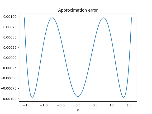
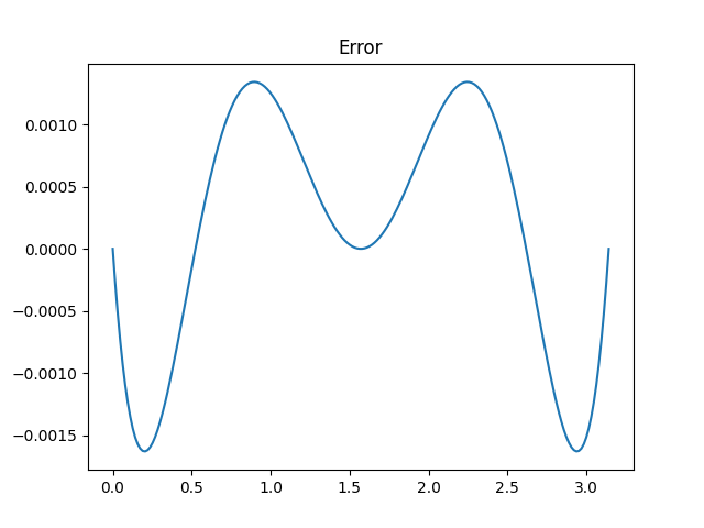
Determining fundamental frequency

My daughter had a homework problem the other day that gave the frequencies of several Fourier components and asked her to find the fundamental frequency. The numbers were nice enough that brute force worked, and I’m sure that’s what students were expected to do. But this could easily be a much more sophisticated problem.

If the frequencies are all integers and exact multiples of a fundamental frequency, you can simply take the greatest common divisor of the frequencies. If you’re told the frequencies are 1760, 2200, and 3080, then the fundamental frequency is apparently 440 since that’s the greatest common divisor.

But what if the data are a little different? Say the highest pitch is 3081. Surely 440 should still be considered the fundamental frequency, even though now the greatest common divisor of the frequencies would be 1 Hz. What if the highest frequency was 3078 + π? Surely the fundamental frequency is still 440 for practical purposes.

And what might these practical purposes be? One purpose might be pitch detection. When several frequencies are combined that are small integer multiples of a fundamental frequency, we perceive the combination as having pitch given by that fundamental.

For something like a guitar string, the frequency components are close to small integer multiples of a fundamental frequency. But for something like a church bell, the frequencies don’t line up so neatly, though there’s still a clearly perceived pitch. For something like a metal mixing bowl, it may be difficulty to predict what pitch a person will hear when something strikes the bowl.

One complication we haven’t addressed yet is that the fundamental frequency will not be unique without some constraint. In the example above, the frequencies were all multiples of 440, but they’re also all multiples of 440/n for every positive integer n. We might get around this by specifying some lower bound on the fundamental frequency. Or we could say that all other things being equal, we want the largest candidate for the fundamental frequency.

We could formulate the problem of finding the fundamental frequency as an optimization problem. For example, we could form a mixed integer program. Suppose we have three frequencies f1, f2, and f3. We could find a fundamental frequency f and integers n1, n2, and n3 that minimize

(f1n1 f)² + (f2n2 f)² + (f3n3 f

subject to a lower bound on f.

We can eliminate the explicit dependence on the integer coefficients by minimizing

(f1/f – [f1/f])² + (f2/f – [f2/f])² + (f3/f – [f3/f])² .

where [x] denotes nearest integer to x. The first formulation has a more common form. The latter has a more complicated objective function, but it’s only a function of one variable.

Here’s what the latter looks like for frequencies 1760, 2200, and 3080.

objective function

Clearly there’s a minimum at 440 Hz.

Here’s the same plot with 10% random noise [1] added to each frequency: 1701, 2368, and 3339.

objective function

Now there’s a minimum near 336, but the local minimum at 566 is nearly as good.

Related posts

[1] There are a couple reasons you might want to solve a problem like this. Maybe your frequencies really are integer multiples of a fundamental frequency, but there is measurement error. Another is that the frequencies are not exactly multiples of a fundamental, as when striking a bell or a mixing bowl. How might you formulate the two cases differently?

Optimization, Dominoes, and Frankenstein

Robert Bosch has a new book coming out next week titled OPT ART: From Mathematical Optimization to Visual Design. This post will look at just one example from the book: creating images of Frankenstein’s monster [1] using dominoes.

Frankenstein made from 3 sets of double nine dominoes

The book includes two images, a low-resolution image made from 3 sets of dominoes and a high resolution image made from 48 sets. These are double nine dominoes rather than the more common double six dominoes because the former allow a more symmetric arrangement of dots. There are 55 dominoes in a double nine set. (Explanation and generalization here.)

Image of Frankenstein's monster made from 48 sets of double nine dominoes

The images are created by solving a constrained optimization problem. You basically want to use dominoes whose brightness is proportional to the brightness of the corresponding section of a photograph. But you can only use the dominoes you have, and you have to use them all.

You would naturally want to use double nines for the brightest areas since they have the most white spots and double blanks for the darkest areas. But you only have three of each in the first image, forty eight of each in the second, and you have to make do with the rest of the available pieces. So you solve an optimization problem to do the best you can.

Each domino can be places horizontally or vertically, as long as they fit the overall shape of the image. In the first image, you can see the orientation of the pieces if you look closely. Here’s a little piece from the top let corner.

Domino orientation

One double six is placed vertically in the top left. Next to it are another double six and a double five placed horizontally, etc.

There are additional constraints on the optimization problem related to contrast. You don’t just want to match the brightness of the photograph as well as you can, you also want to maintain contrast. For example, maybe a five-two domino would match the brightness of a couple adjacent squares in the photograph, but a seven-one would do a better job of making a distinction between contrasting regions of the image.

Bosch explains that the problem statement for the image using three sets of dominoes required 34,265 variables and 385 domino constraints. It was solved using 29,242 iterations of a simplex algorithm and required a little less than 2 seconds.

The optimization problem for the image created from 48 sets of dominoes required 572,660 variables and 5,335 constraints. The solution required 30,861 iterations of a simplex algorithm and just under one minute of computation.

Related posts

[1] In the Shelley’s novel Frankenstein, the doctor who creates the monster is Victor Frankenstein. The creature is commonly called Frankenstein, but strictly speaking that’s not his name. There’s a quote—I haven’t been able to track down its source—that says “Knowledge is knowing that Frankenstein wasn’t the monster. Wisdom is knowing that Frankenstein was the monster.” That is, the monster’s name wasn’t Frankenstein, but what Victor Frankenstein did was monstrous.

Something that bothers me about deep neural nets

Overfitting happens when a model does too good a job of matching a particular data set and so does a poor job on new data. The way traditional statistical models address the danger of overfitting is to limit the number of parameters. For example, you might fit a straight line (two parameters) to 100 data points, rather than using a 99-degree polynomial that could match the input data exactly and probably do a terrible job on new data. You find the best fit you can to a model that doesn’t have enough flexibility to match the data too closely.

Deep neural networks have enough parameters to overfit the data, but there are various strategies to keep this from happening. A common way to avoid overfitting is to deliberately do a mediocre job of fitting the model.

When it works well, the shortcomings of the optimization procedure yield a solution that differs from the optimal solution in a beneficial way. But the solution could fail to be useful in several ways. It might be too far from optimal, or deviate from the optimal solution in an unhelpful way, or the optimization method might accidentally do too good a job.

It a nutshell, the disturbing thing is that you have a negative criteria for what constitutes a good solution: one that’s not too close to optimal. But there are a lot of ways to not be too close to optimal. In practice, you experiment until you find an optimally suboptimal solution, i.e. the intentionally suboptimal fit that performs the best in validation.


One of my favorite proofs: Lagrange multipliers

One of my lightbulb moments in college was when my professor, Jim Vick, explained the Lagrange multiplier theorem. The way I’d seen it stated in a calculus text gave me no feel for why it should be true, but his explanation made sense immediately.

Suppose f(x) is a function of several variables, i.e. x is a vector, and g(x) = c is a constraint. Then the Lagrange multiplier theorem says that at the maximum of f subject to the constraint g we have ∇f = λ ∇g.

Where does this mysterious λ come from? And why should the gradient of your objective function be related to the gradient of a constraint? These seem like two different things that shouldn’t even be comparable.

Here’s the geometric explanation. The set of points satisfying g(x) = c is a surface. And for any k, the set of points satisfying f(x) = k is also surface. Imagine k very large, larger than the maximum of f on the surface defined by g(x) = c. You could think of the surface g(x) = c being a balloon inside the larger balloon  f(x) = k.

Now gradually decrease k, like letting the air out of the outer balloon, until the surfaces g(x) = c and f(x) = k first touch. At that point, the two surfaces will be tangent, and so their normal vectors, given by their gradients, point in the same direction. That is, ∇f and ∇g are parallel, and so ∇f is some multiple of ∇g. Call that multiple λ.

I don’t know how well that explanation works when written down. But when I heard Jim Vick explain it, moving his hands in the air, it was an eye-opener.

This is not a rigorous proof, and it does not give the most general result possible, but it explains what’s going on. It’s something to keep in mind when reading proofs that are more rigorous or more general. As I comment on here,

Proofs serve two main purposes: to establish that a proposition is true, and to show why it is true.

The literally hand-wavy proof scores low on the former criterion and high on the latter.

***

Jim Vick was a great teacher. Some of us affectionately called him The Grinning Demon because he was always smiling, even while he gave devilishly hard homework. He was Dean of Natural Sciences when I took a couple classes from him. He later became Vice President for Student Affairs and kept teaching periodically. He has since retired but still teaches.

After taking his topology course, several of us asked him to teach a differential geometry course. He hesitated because it’s a challenge to put together an undergraduate differential geometry course. The usual development of differential geometry uses so much machinery that it’s typically a graduate-level course.

Vick found a book that starts by looking only at manifolds given by level sets of smooth functions, like the surfaces discussed above. Because these surfaces sit inside a Euclidean space, you can quickly get to some interesting geometric results using elementary methods. We eventually got to the more advanced methods, but by then we had experience in a more tangible setting. As Michael Atiyah said, abstraction should follow experience, not precede it.

Natural optima occur in the middle

Akin’s eighth law of spacecraft design says

In nature, the optimum is almost always in the middle somewhere. Distrust assertions that the optimum is at an extreme point.

When I first read this I immediately thought of several examples where theory said that an optima was at an extreme, but experience said otherwise.

Linear programming (LP) says the opposite of Akin’s law. The optimal point for a linear objective function subject to linear constraints is always at an extreme point. The constraints form a many-sided shape—you could think of it something like a diamond—and the optimal point will always be at one of the corners.

Nature is not linear, though it is often approximately linear over some useful range. One way to read Akin’s law is to say that even when something is approximately linear in the middle, there’s enough non-linearity at the extremes to pull the optimal points back from the edges. Or said another way, when you have an optimal value at an extreme point, there may be some unrealistic aspect of your model that pushed the optimal point out to the boundary.

Related postData calls the model’s bluff