Random walks mix faster on some graphs than on others. Rapid mixing is one of the ways to characterize expander graphs.
By rapid mixing we mean that a random walk approaches its limiting (stationary) probability distribution quickly relative to random walks on other graphs.
Here’s a graph that supports rapid mixing. Pick a prime p and label nodes 0, 1, 2, 3, …, p − 1. Create a circular graph by connecting each node k to (k + 1) mod p. Then add an edge between each non-zero k to its multiplicative inverse mod p. If an element is its own inverse, add a loop connecting the node to itself. For the purpose of this construction, consider 0 to be its own inverse. This construction comes from [1].
Here’s what the graph looks like with p = 23.
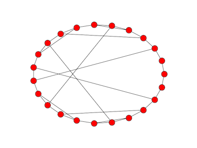
This graph doesn’t show the three loops from a node to itself, nodes 1, 0, and 22.
At each node in the random walk, we choose an edge uniformly and follow it. The stationary distribution for a random walk on this graph is uniform. That is, in the long run, you’re equally likely to be at any particular node.
If we pick an arbitrary starting node, 13, and take 30 steps of the random walk, the simulated probability distribution is nearly flat.

By contrast, we take a variation on the random walk above. From each node, we move left, right, or stay in place with equal probability. This walk is not as well mixed after 100 steps as the original walk is after only 30 steps.

You can tell from the graph that the walk started around 13. In the previous graph, evidence of the starting point had vanished.
The code below was used to produce these graphs.
To investigate how quickly a walk on this graph converges to its limiting distribution, we could run code like the following.
    from random import random
    import numpy as np
    import matplotlib.pyplot as plt
    m = 23

    # Multiplicative inverses mod 23
    inverse = [0, 1, 12, 8, 6, 14, 4, 10, 3, 18, 7, 21, 2, 16, 5, 20, 13, 19, 9, 17, 15, 11, 22]

    # Verify that the inverses are correct
    assert(len(inverse) == m)
    for i in range(1, m):
        assert (i*inverse[i] % 23 == 1)

    # Simulation
    num_reps = 100000
    num_steps = 30

    def take_cayley_step(loc):
        u = random() * 3
        if u < 1: # move left
            newloc = (loc + m - 1) % m
        elif u < 2: # move right
            newloc = (loc + 1) % m
        else:
            newloc = inverse[loc] # or newloc = loc
        return newloc

    stats = [0]*m
    for i in range(num_reps):
        loc = 13 # arbitrary fixed starting point
        for j in range(num_steps):
            loc = take_cayley_step(loc)
        stats[loc] += 1

    normed = np.array(stats)/num_reps
    plt.plot(normed)
    plt.xlim(1, m)
    plt.ylim(0,2/m)
    plt.show()
Related posts
* * *
[1] Shlomo Hoory, Nathan Linial, Avi Wigderson. “Expander graphs and their applications.” Bulletin of the American Mathematical Society, Volume 43, Number 4, October 2006, pages 439–561.