Monthly highlights

Posted on 9 January 2017 by John

If you enjoy reading the articles here, you might like a monthly review of the most popular posts.

I send out a newsletter at the end of each month. I’ve sent out around 20 so far. They all have two parts:

a review of the most popular posts of the month, and
a few words about what I’ve been up to.

That’s it. Short and sweet. I might send out more mail than this someday, but I’ve been doing this for nearly two years I’ve never sent more than one email a month.

If you’d like to subscribe, just enter your email address in the box on the side of the page labeled “Subscribe to my newsletter.” If you’re not reading this directly on the site, say you’re reading it in an RSS reader, then you can follow this link.

Cover time of a graph: cliques, chains, and lollipops

Posted on 4 January 2017 by John

Cover time

The cover time of a graph is the expected time it takes a simple random walk on the graph to visit every node. A simple random walk starts at some node, then at each step chooses with equal probability one of the adjacent nodes. The cover time is defined to be the maximum over all starting points of expected time to visit all nodes.

It seems plausible that adding edges to a graph would decrease its cover time. Sometimes this is the case and sometimes it isn’t, as we’ll demonstrate below.

Chains, complete graphs, and lollipops

This post will look at three kinds of graphs

a chain of n vertices
a complete graph on n vertices
a “lollipop” with n vertices

A chain simply connects vertices in a straight line. A complete graph connects every node to every other node.

A lollipop graph of order (5, 5)

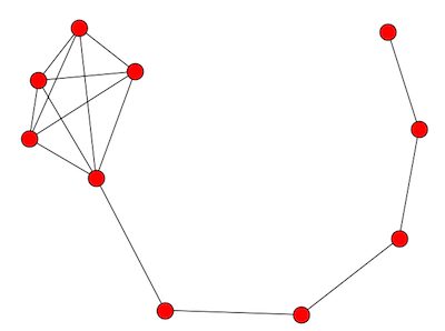
A lollipop with n vertices takes a chain with n/2 vertices and complete graph on n/2 vertices and joins them together. The image above is a lollipop graph of order 10. The complete graph becomes a clique in the new graph.

The image looks more like a kite than a lollipop because that’s the way my software (networkx) drew it by default. If you’d like, image the complete graph more round and the chain more straight so that the graph more closely resembles a lollipop.

Random walks on graphs

Chains have a long cover time. Complete graphs have a short cover time. What about lollipops?

A plausible answer would be that a lollipop graph would have a moderate cover time, somewhere between that of a complete graph and a chain. But that’s not the case. In fact, the lollipop has a longer cover time than either the complete graph or the chain.

You could think of a lollipop graph with n vertices as a chain of length n with extra edges added. This shows that adding edges does not always decrease the cover time.

The cover times for the three graphs we consider here are of different orders: O(n log n) for the complete graph, O(n²) for the chain, and O(n³) for the lollipop.

Now these are only asymptotic results. Big-O notation leaves out proportionality constants. We know that for sufficiently large n the cover times are ordered so that the complete graph is the smallest, then the chain, then the lollipop. But does n have to be astronomically large before this happens? What happens with a modest size n?

There’s a theoretical result that says the cover time is bounded by 2m(n − 1) where m is the number of edges and n the number of vertices. This tells us that when we say the cover time for the chain is O(n²) we can say more, that it’s less than 2n², so at least in this case the proportionality constant isn’t large.

We’ll look at the cover times with some simulation results below based on n = 10 and n = 30 based on 10,000 runs.

With 10 nodes each, the cover times for the complete graph, chain, and lollipop were 23.30, 82.25, and 131.08 respectively.

With 30 nodes the corresponding cover times were 114.37, 845.16, and 3480.95.

So the run times were ordered as the asymptotic theory would suggest.

Changing names

Posted on 3 January 2017 by John

I’ve just started reading Laurus, an English translation of a contemporary Russian novel. The book opens with this paragraph.

He had four names at various times. A person’s life is heterogeneous, so this could be seen as an advantage. Life’s parts sometimes have little in common, so little that it might appear that various people lived them. When this happens, it is difficult not to feel surprised that all these people carry the same name.

This reminded me of the section of James Scott’s Seeing Like a State that explains how names used to be more variable.

Among some peoples, it is not uncommon for individuals to have different names during different stages of life (infancy, childhood, adulthood) and in some cases after death; added to these are names used for joking, rituals, and mourning and names used for interactions with same-sex friends or with in-laws. Each name is specific to a certain phase of life, social setting, or interlocutor.

If someone’s name had more than one component, the final component might come from their profession (which could change) rather than their ancestry. Scott goes on to say

The invention of permanent, inherited patronyms was … the last step in establishing the necessary preconditions of modern statecraft. In almost every case it was a state project, designed to allow officials to identify, unambiguously, the majority of its citizens.

In short, governments insisted people adopt fixed names to make them easier to tax and to conscript. Before fixed names, governments would ask towns to provide so much tax money or so many soldiers because it could not tax or conscript citizens directly. For a famous example, see Luke’s account of the birth of Jesus: all went to be registered, each to his own town.

It’s hard to imagine people not needing fixed names. But when people lived on a smaller scale, interacting with a number of people closer to Dunbar’s number, there was no danger of ambiguity because there was more context.

Bernoulli numbers, Riemann zeta, and strange sums

Posted on 3 January 2017 by John

In the previous post, we looked at sums of the first n consecutive powers, i.e. sums of the form

$S_p(n) = \sum_{k=1}^n k^p$

where p was a positive integer. Here we look at what happens when we let p be a negative integer and we let n go to infinity. We’ll learn more about Bernoulli numbers and we’ll see what is meant by apparently absurd statements such as 1 + 2 + 3 + … = −1/12.

If p < −1, then the limit as n goes to infinity of S_p(n) is ζ(−p). That is, for s > 1, the Riemann zeta function ζ(s) is defined by

$\zeta(s) = \sum_{n=1}^\infty \frac{1}{n^s}$

We don’t have to limit ourselves to real numbers s > 1; the definition holds for complex numbers s with real part greater than 1. That’ll be important below.

When s is a positive even number, there’s a formula for ζ(s) in terms of the Bernoulli numbers:

$\zeta(2n) = (-1)^{n-1} 2^{2n-1} \pi^{2n} \frac{B_{2n}}{(2n)!}$

The best-known special case of this formula is that

1 + 1/4 + 1/9 + 1/16 + … = π² / 6.

It’s a famous open problem to find a closed-form expression for ζ(3) or any other odd argument.

The formula relating the zeta function and Bernoulli tells us a couple things about the Bernoulli numbers. First, for n ≥ 1 the Bernoulli numbers with index 2n alternate sign. Second, by looking at the sum defining ζ(2n) we can see that it is approximately 1 for large n. This tells us that for large n, |B_2n| is approximately (2n)! / 2²ⁿ⁻¹ π²ⁿ.

We said above that the sum defining the Riemann zeta function is valid for complex numbers s with real part greater than 1. There is a unique analytic extension of the zeta function to the rest of the complex plane, except at s = 1. The zeta function is defined, for example, at negative integers, but the sum defining zeta in the half-plane Re(s) > 1 is NOT valid.

You may have seen the equation

1 + 2 + 3 + … = −1/12.

This is an abuse of notation. The sum on the left clearly diverges to infinity. But if the sum defining ζ(s) for Re(s) > 1 were valid for s = −1 (which it is not) then the left side would equal ζ(−1). The analytic continuation of ζ is valid at -1, and in fact ζ(−1) = −1/12. So the equation above is true if you interpret the left side, not as an ordinary sum, but as a way of writing ζ(−1). The same approach could be used to make sense of similar equations such as

1² + 2² + 3² + … = 0

and

1³ + 2³ + 3³ + … = 1/120.

Related: Posts on special numbers

Month: January 2017