Last year I wrote a post about saxophone octave keys. I was surprised to discover, after playing saxophone for most of my life, that a saxophone has not one but two octave holes. Modern saxophones have one octave key, but two octave holes. Originally saxophones had a separate octave key for each octave hole; you had to use different octave keys for different notes.
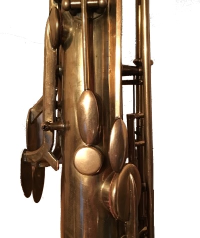
I had not seen one of these old saxophones until Carlo Burkhardt sent me photos today of a Pierret Modele 5 Tenor Sax from around 1912.
Here’s a closeup of the octave keys.
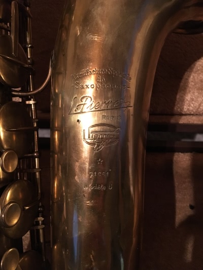
And here’s a closeup of the bell where you can see the branding.
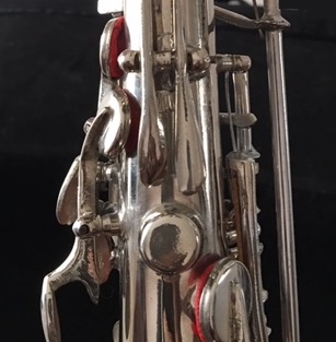
Update (2019-01-22): A reader, Paul A., sent me photos of a silver alto sax with two octave keys. More on this saxophone here.
The other day I wrote about the golden angle, a variation on the golden ratio. If φ is the golden ratio, then a golden angle is 1/φ2 of a circle, approximately 137.5°, a little over a third of a circle.
Musical notes go around in a circle. After 12 half steps we’re back where we started. What would it sound like if we played intervals that went around this circle at golden angles? I’ll include audio files and the code that produced them below.
A golden interval, moving around the music circle by a golden angle, is a little more than a major third. And so a chord made of golden intervals is like an augmented major chord but stretched a bit.
An augmented major triad divides the musical circle exactly in thirds. For example, C E G#. Each note is four half steps, a major third, from the previous note. In terms of a circle, each interval is 120°. Here’s what these notes sound like in succession and as a chord.
If we go around the musical circle in golden angles, we get something like an augmented triad but with slightly bigger intervals. In terms of a circle, each note moves 137.5° from the previous note rather than 120°. Whereas an augmented triad goes around the musical circle at 0°, 120°, and 240° degrees, a golden triad goes around 0°, 137.5°, and 275°.
A half step corresponds to 30°, so a golden angle corresponds to a little more than 4.5 half steps. If we start on C, the next note is between E and F, and the next is just a little higher than A.
If we keep going up in golden intervals, we do not return to the note we stared on, unlike a progression of major thirds. In fact, we never get the same note twice because a golden interval is not a rational part of a circle. Four golden angle rotations amount to 412.5°, i.e. 52.5° more than a circle. In terms of music, going up four golden intervals puts us an octave and almost a whole step higher than we stared.
Here’s what a longer progression of golden intervals sounds like. Each note keeps going but decays so you can hear both the sequence of notes and how they sound in harmony. The intention was to create something like playing the notes on a piano with the sustain pedal down.
It sounds a little unusual but pleasant, better than I thought it would.
Here’s the Python code that produced the sound files in case you’d like to create your own. You might, for example, experiment by increasing or decreasing the decay rate. Or you might try using richer tones than just pure sine waves.
from scipy.constants import golden
import numpy as np
from scipy.io.wavfile import write

N = 44100 # samples per second

# Inputs:
# frequency in cycles per second
# duration in seconds
# decay = half-life in seconds
def tone(freq, duration, decay=0):
    t = np.arange(0, duration, 1.0/N)
    y = np.sin(freq*2*np.pi*t)
    if decay > 0:
        k = np.log(2) / decay
        y *= np.exp(-k*t)
    return y

# Scale signal to 16-bit integers,
# values between -2^15 and 2^15 - 1.
def to_integer(signal):
    signal /= max(abs(signal))
    return np.int16(signal*(2**15 - 1))

C = 262 # middle C frequency in Hz

# Play notes sequentially then as a chord
def arpeggio(n, interval):
    y = np.zeros((n+1)*N)
    for i in range(n):
        x = tone(C * interval**i, 1)
        y[i*N : (i+1)*N] = x
        y[n*N : (n+1)*N] += x
    return y

# Play notes sequentially with each sustained
def bell(n, interval, decay):
    y = np.zeros(n*N)
    for i in range(n):
        x = tone(C * interval**i, n-i, decay)
        y[i*N:] += x
    return y

major_third = 2**(1/3)
golden_interval = 2**(golden**-2)

write("augmented.wav", N, to_integer(arpeggio(3, major_third)))

write("golden_triad.wav", N, to_integer(arpeggio(3, golden_interval)))

write("bell.wav", N, to_integer(bell(9, golden_interval, 6)))
Here’s a script I wanted to write: given a color c specified in RGB and an angle θ, rotate c on the color wheel by θ and return the RGB value of the result.
You can’t rotate RGB values per se, but you can rotate hues. So my initial idea was to convert RGB to HSV or HSL, rotate the H component, then convert back to RGB. There are some subtleties with converting between RGB and either HSV or HSL, but I’m willing to ignore those for now.
The problem I ran into was that my idea of a color wheel doesn’t match the HSV or HSL color wheels. For example, I’m thinking of green as the complementary color to red, the color 180° away. On the HSV and HSL color wheels, the complementary color to red is cyan. The color wheel I have in mind is the “artist’s color wheel” based on the RYB color space, not RGB. Subtractive color, not additive.
This brings up several questions.
How do you convert back and forth between RYB and RGB?
How do you describe the artist’s color wheel mathematically, in RYB or any other system?
What is a good reference on color theory? I’d like to understand in detail how the various color systems relate, something that spans the gamut (pun intended) from an artist’s perspective down to physics and physiology.
“Teachers should prepare the student for the student’s future, not for the teacher’s past.” — Richard Hamming
I ran across the above quote from Hamming this morning. It made me wonder whether I tried to prepare students for my past when I used to teach college students.
How do you prepare a student for the future? Mostly by focusing on skills that will always be useful, even as times change: logic, clear communication, diligence, etc.
Negative forecasting is more reliable here than positive forecasting. It’s hard to predict what’s going to be in demand in the future (besides timeless skills), but it’s easier to predict what’s probably not going to be in demand. The latter aligns with Hamming’s exhortation not to prepare students for your past.
… in an ideal world, people would learn this material over many years, after having background courses in commutative algebra, algebraic topology, differential geometry, complex analysis, homological algebra, number theory, and French literature.
It is always strange and painful to have to change a habit of mind; though, when we have made the effort, we may find a great relief, even a sense of adventure and delight, in getting rid of the false and returning to the true.
Start with a rose, as described in the previous post:
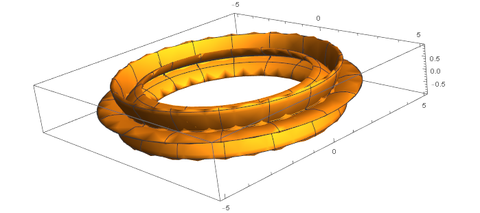
Now spin that rose around a vertical line a distance R from the center of the rose. This makes a torus (doughnut) shape whose cross sections look like the rose above. You could think of having a cutout shaped like the rose above and extruding Play-Doh through it, then joining the ends in a loop.
In case you’re curious, the image above was created with the following Mathematica command:
This sounds like a horrendous calculus homework problem, but it’s actually quite easy. A theorem by Pappus of Alexandria (c. 300 AD) says that the volume is equal to the area times the circumference of the circle traversed by the centroid.
The area of a rose of the form r = cos(kθ) is simply π/2 if k is even and π/4 if k is odd. (Recall from the previous post that the number of petals is 2k if k is even and k if k is odd.)
The location of the centroid is easy: it’s at the origin by symmetry. If we rotate the rose around a vertical line x = R then the centroid travels a distance 2πR.
So putting all the pieces together, the volume is π²R if k is even and half that if k is odd. (We assume R > 1 so that the figure doesn’t intersect itself and some volume get counted twice.)
We can also find the surface area easily by another theorem of Pappus. The surface area is just the arc length of the rose times the circumference of the circle traced out by the centroid. The previous post showed how to find the arc length, so just multiply that by 2πR.
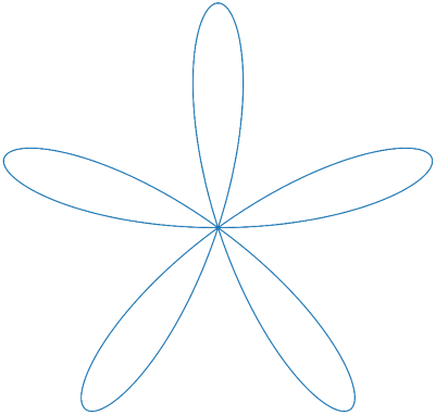
The polar graph of r = cos(kθ) is called a rose. If k is even, the curve will trace out 2k petals as θ runs between 0 and 2π. If k is odd, it will trace out k petals, tracing each one twice. For example, here’s a rose with k = 5.
(I rotated the graph 36° so it would be symmetric about the vertical axis rather than the horizontal axis.)
The arc length of a curve in polar coordinates is given by
and so we can use this find the length. The integral doesn’t have a closed form in terms of elementary functions. Instead, the result turns out to use a special function E(x), the “complete elliptic integral of the second kind,” defined by
Here’s the calculation for the length of a rose:
So the arc length of the rose r = cos(kθ) with θ running from 0 to 2π is 4 E(−k² + 1). You can calculate E in SciPy with scipy.special.ellipe.
If we compute the length of the rose at the top of the post, we get 4 E(−24) = 21.01. Does that pass the sniff test? Each petal goes from r = 0 out to r = 1 and back. If the petal were a straight line, this would have length 2. Since the petals are curved, the length of each is a little more than 2. There are five petals, so the result should be a little more than 10. But we got a little more than 20. How can that be? Since 5 is odd, the rose with k = 5 traces each petal twice, so we should expect a value of a little more than 20, which is what we got.
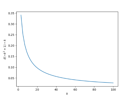
As k gets larger, the petals come closer to being straight lines. So we should expect that 4E(−k² + 1) approaches 4k as k gets large. The following plot of E(−k² + 1) – k provides empirical support for this conjecture by showing that the difference approaches 0, and gives an idea of the rate of convergence. It should be possible to prove that, say, that E(−k²) asymptotically approaches k, but I haven’t done this.
The graph of hyperbolic cosine is called a catenary. A catenary has the following curious property: the length of a catenary between two points equals the area under the catenary between those two points.
The proof is surprisingly simple. Start with the following:
Now integrate the first and last expressions between two points a and b. Note that the former integral gives the arc length of cosh between a and b, and the later integral gives the area under the graph of cosh between a and b.
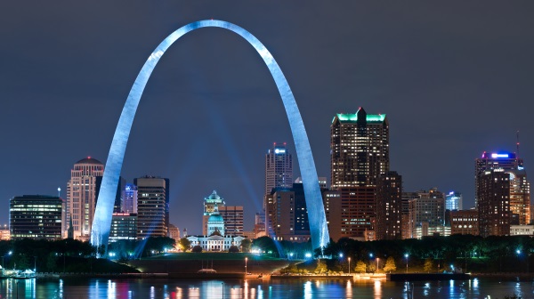
By the way, the most famous catenary may be the Gateway Arch in St. Louis, Missouri.