Gamma function partial sums

Last week I wrote about Jentzsch’s theorem. It says that if the power series of function has a finite radius of convergence, the set of zeros of the partial sums of the series will cluster around and fill in the boundary of convergence.

This post will look at the power series for the gamma function centered at 1 and will use a different plotting style.

Here’s what the contours look like with 12 terms:

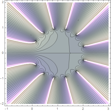
The radius of convergence is 1 because the gamma function has a singularity at 0. (The radius of convergence is the distance from the center of the power series to the nearest singularity.) Contour lines correspond to constant phase. The gamma function is real for real arguments, and so you can see the real axis running through the middle of the plot because real numbers have zero phase. The contour lines meet at zeros, which you can see are near a circle of radius 1 centered at z = 1.

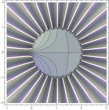
Here’s what the contour plot looks like with 30 terms:

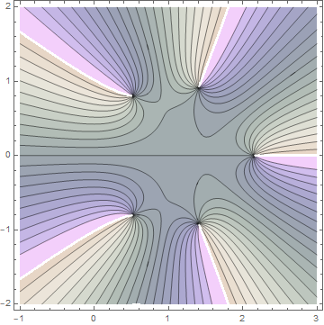
And here’s what it looks like with just 5 terms:

Here’s the Mathematica code that was used to create the images.

    P[x_] = Normal[Series[1.0 Gamma[x], {x, 1, 12}]]
    ContourPlot[
        Arg[P[x + I y]], 
        {x, -1, 3}, 
        {y, -2, 2}, 
        ColorFunction -> "PearlColors", 
        Contours -> 20
    ]

The 1.0 in front of the call to Gamma is important. It tells Mathematica to numerically evaluate the coefficients of the power series. Otherwise Mathematica will find the coefficients symbolically and the plots will take forever.

Similarly, the call to Normal tells Mathematica not to carry around a symbolic error term O(x - 1)13.