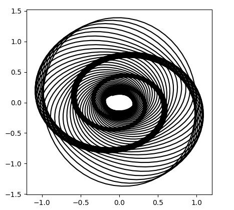
In the previous post, I said that Lissajous curves are the result of plotting a curve whose x and y coordinates come from (undamped) harmonic oscillators. If we add a little bit of dampening, multiplying our cosine terms by negative exponentials, the resulting curve is called a harmonograph.
Here’s a bit of Mathematica code to draw harmonographs.
harmonograph[f1_, f2_, ph1_, ph2_, d1_, d2_, T_] :=
    ParametricPlot[{
        Cos[f1 t + ph1] Exp[-d1 t],
        Cos[f2 t + ph2] Exp[-d2 t]
    }, {t, 0, T}]
For example,
harmonograph[3, 4, 0, Sqrt[2], 0.01, 0.02, 100]
is a slight variation on one of the curves from the previous post, adding dampening terms exp(-0.01t) and exp(-0.01t). The result is the following.
You can get a wide variety of graphs by playing with the parameters. A couple years ago I wrote about an attempt to reproduce the background of the image in the poster for Alfred Hitchcock’s movie Vertigo. The curve is another example of a harmonograph.