Expected value of X and 1/X

Yesterday I blogged about an exercise in the book The Cauchy-Schwarz Master Class. This post is about another exercise from that book, exercise 5.8, which is to prove Kantorovich’s inequality.

Assume

0 < m \leq x_1 \leq x_2 \leq \cdots \leq x_n \leq M < \infty

and

p_1 + p_2 + \cdots + p_n = 1

for non-negative numbers pi.

Then

\left(\sum_{i=1}^n p_i x_i \right) \left(\sum_{i=1}^n p_i \frac{1}{x_i} \right) \leq \frac{\mu^2}{\gamma^2}

where

\mu = \frac{m+M}{2}

is the arithmetic mean of m and M and

\gamma = \sqrt{mM}

is the geometric mean of m and M.

In words, the weighted average of the x‘s times the weighted average of their reciprocals is bounded by the square of the ratio of the arithmetic and geometric means of the x‘s.

Probability interpretation

I did a quick search on Kantorovich’s inequality, and apparently it first came up in linear programming, Kantorovich’s area of focus. But when I see it, I immediately think expectations of random variables. Maybe Kantorovich was also thinking about random variables, in the context of linear programming.

The left side of Kantorovich’s inequality is the expected value of a discrete random variable X and the expected value of 1/X.

To put it another way, it’s a relationship between E[1/X] and 1/E[X],

\text{E}\left(\frac{1}{X} \right ) \leq \frac{\mu^2}{\gamma^2} \frac{1}{\text{E}(X)}

which I imagine is how it is used in practice.

I don’t recall seeing this inequality used, but it could have gone by in a blur and I didn’t pay attention. But now that I’ve thought about it, I’m more likely to notice if I see it again.

Python example

Here’s a little Python code to play with Kantorovich’s inequality, assuming the random values are uniformly distributed on [0, 1].

    from numpy import random

    x = random.random(6)
    m = min(x)
    M = max(x)
    am = 0.5*(m+M)
    gm = (m*M)**0.5
    prod = x.mean() * (1/x).mean()
    bound = (am/gm)**2
    print(prod, bound)

This returned 1.2021 for the product and 1.3717 for the bound.

If we put the code above inside a loop we can plot the product and its bound to get an idea how tight the bound is typically. (The bound is perfectly tight if all the x’s are equal.) Here’s what we get.

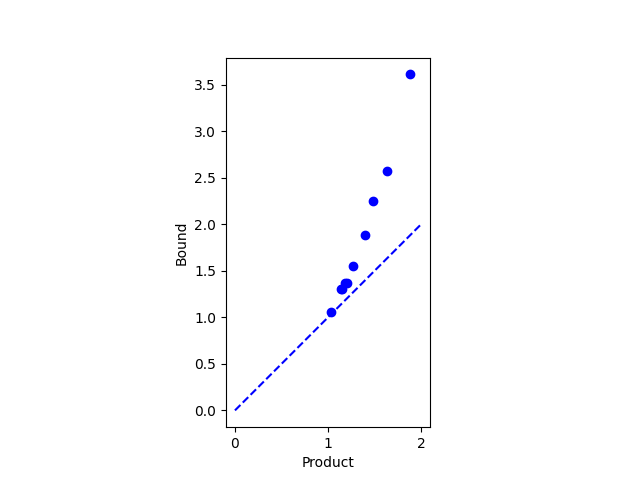
All the dots are above the dotted line, so we haven’t found an exception to our inequality.

(I didn’t think that Kantorovich had made a mistake. If he had, someone would have noticed by now. But it’s worth testing a theorem you know to be true, in order to test that your understanding of the theorem is correct.)

More inequalities

The baseball inequality

baseball game

There’s a theorem that’s often used and assumed to be true but rarely stated explicitly. I’m going to call it “the baseball inequality” for reasons I’ll get to shortly.

Suppose you have two lists of k positive numbers each:

n_1, n_2, n_3, \ldots, n_k

and

d_1, d_2, d_3, \ldots, d_k

Then

\min_{1 \leq i \leq k} \frac{n_i}{d_i} \leq \frac{n_1 + n_2 + n_3 + \cdots + n_k}{d_1 + d_2 + d_3 + \cdots + d_k} \leq \max_{1 \leq i \leq k} \frac{n_i}{d_i}

This says, for example, that the batting average of a baseball team is somewhere between the best individual batting average and the worst individual batting average.

The only place I can recall seeing this inequality stated is in The Cauchy-Schwarz Master Class by Michael Steele. He states the inequality in exercise 5.1 and gives it the batting average interpretation. (Update: This is known as the “mediant inequality.” Thanks to Tom in the comments for letting me know. So the thing in the middle is called the “mediant” of the fractions.)

Note that this is not the same as saying the average of a list of numbers is between the smallest and largest numbers in the list, though that’s true. The batting average of a team as a whole is not the same as the average of the individual batting averages on that team. It might happen to be, but in general it is not.

I’ll give a quick proof of the baseball inequality. I’ll only prove the first of the two inequalities. That is, I’ll prove that the minimum fraction is no greater than the ratio of the sums of numerators and denominators. Proving that the latter is no greater than the maximum fraction is completely analogous.

Also, I’ll only prove the theorem for two numerators and two denominators. Once you have proved the inequality for two numerators and denominators, you can bootstrap that to prove the inequality for three numerators and three denominators, and continue this process for any number of numbers on top and bottom.

So we start by assuming

\frac{a}{b} \leq \frac{c}{d}

Then we have

\begin{align*} \frac{a}{b} &= \frac{a\left(1 + \dfrac{d}{b} \right )}{b\left(1 + \dfrac{d}{b} \right )} \\ &= \frac{a + \dfrac{a}{b}d}{b + d} \\ &\leq \frac{a + \dfrac{c}{d}d}{b+d} \\ &= \frac{a + c}{b+d} \end{align*}

More inequality posts