The geometric, logarithmic, and arithmetic means of a and b are defined as follows.

A few days ago I mentioned that G ≤ L ≤ A. The logarithmic mean slips between the geometric and arithmetic means.

Or to put it another way, the logarithmic mean is bounded by the geometric and arithmetic means. You can bound the logarithmic mean more tightly with a mixture of the geometric and arithmetic means.

In [1] the authors show that

Note that the leftmost expression is the geometric mean of G, G, and A, and the rightmost expression is the arithmetic mean of G, G, and A. We can write this as

where G with no argument is the geometric mean of a and b and G with three arguments is the geometric mean of those arguments, and similarly for A.

The following plot shows how well these means of means bound the logarithmic mean. We let a = 1 and let b vary from 1 to 10o.

The upper bound is especially tight for moderate values of b. When I first made the plot I let b run up to 10 and there were apparently only four curves in the plot. I had to pick a larger value of b before the curves for L and (2G + A)/3 to be distinguished.

Related posts

• Integral representations of means
• Sierpiński’s inequality
• Extending AGM to three variables

[1] Graham Jameson and Peter R. Mercer. The Logarithmic Mean Revisited. The American Mathematical Monthly, Vol. 126, No. 7, pp. 641-645

Let

with each component satisfying 0 < x_i ≤ 1/2. Define the complement x′ by taking the complement of each entry.

Let G and A represent the geometric and arithmetic mean respectively.

Then Ky Fan’s inequality says

Now let H be the harmonic mean. Since in general H ≤ G ≤ A, you might guess that Ky Fan’s inequality could be extended to

and indeed this is correct.

Source: Jósef Sándor. Theory and Means and Their Inequalities.

The average of two numbers, a and b, can be written as the average of x over the interval [a, b]. This is easily verified as follows.

The average is the arithmetic mean. We can represent other means as above if we generalize the pattern to be

For the arithmetic mean, φ(x) = x.

Logarithmic mean

If we set φ(x) = 1/x we have

and the last expression is known as the logarithmic mean of a and b.

Geometric mean

If we set φ(x) = 1/x² we have

which gives the geometric mean of a and b.

Identric mean

In light of the means above, it’s reasonable ask what happens if we set φ(x) = log x. When we do we get a more arcane mean, known as the identric mean.

The integral representation of the identric mean seems natural, but when we compute the integral we get something that looks arbitrary.

The initial expression looks like something that might come up in application. The final expression looks artificial.

Because the latter is more compact, you’re likely to see the identric mean defined by this expression, then later you might see the integral representation. This is unfortunate since the integral representation makes more sense.

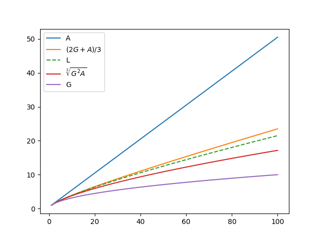
Order of means

It is well known that the geometric mean is no greater than the arithmetic mean. The logarithmic and identric means squeeze in between the geometric and arithmetic means.

If we denote the geometric, logarithmic, identric, and arithmetic means of a and b by G, L, I, and A respectively,

Related posts

• Means of an octave
• Contraharmonic mean
• Geometric mean over unit circle

Let A_n, G_n and H_n be the arithmetic mean, geometric mean, and harmonic mean of a set of n numbers.

When n = 2, the arithmetic mean times the harmonic mean is the geometric mean squared. The proof is simple:

When n > 2 we no longer have equality. However, W. Sierpiński, perhaps best known for the Sierpiński’s triangle, proved that an inequality holds for all n. Given

we have the inequality

Related posts

• Newton’s inequality
• Lehman’s inequality and circuits
• The reversed Cauchy-Schwarz inequality

[1] W. Sierpinski. Sur une inégalité pour la moyenne alrithmétique, géometrique, et harmonique. Warsch. Sitzunsuber, 2 (1909), pp. 354–357.

A few days ago I wrote about sufficient conditions for f(g(x)) to bound g(f(x)). This evening I stumbled on an analogous theorem.

For real numbers γ and δ,

cos(γ sin(x)) > sin(δ cos(x))

for all real x provided

γ² + δ² < (π/2)².

Source: American Mathematical Monthly. February 2009. Solution to problem 11309, page 184.

The reference gives two proofs of the theorem above.

Here’s a quick and dirty Python script that suggests the theorem and its converse are both true.

from numpy import *
import matplotlib.pyplot as plt

N = 200
xs = linspace(0, pi, N)
ds = linspace(-0.5*pi, 0.5*pi, N)
gs = linspace(-0.5*pi, 0.5*pi, N)

def f(x, d, g): return cos(g*sin(x)) - sin(d*cos(x))

for d in ds:
    for g in gs:
        if all(f(xs, d, g) > 0):
            plt.plot(d, g, 'bo')
            if d**2 + g**2 > (pi/2)**2:
                print(d, g)
                
plt.gca().set_aspect("equal")
plt.show()

This produces a big blue disk of radius π/2, confirming that the condition

γ² + δ² < (π/2)²

is sufficient. Furthermore, it prints nothing, which suggests the condition is also necessary.

I stumbled upon a theorem today that I feel like I’ve needed in the past, though I can’t remember any particular applications. I’m writing it up here as a note to my future self should the need reappear.

The theorem gives sufficient conditions to conclude

f(g(x)) ≤ g(f(x))

and uses this to prove, for example, that

arcsin( sinh(x/2) ) ≤ sinh( arcsin(x)/2 )

on the interval [0, 1].

If you think of any applications, please leave a comment.

Here’s the theorem, found in [1].

Let f be continuous with domain 0 ≤ x < 1 or 0 ≤ x ≤ 1, f(0) = 0, f(1) > 1 (including the possibility that f(1) = +∞); let g be continuous with domain the range of f, and g(1) ≤ 1. Let f(x)/x and g(x)/x be strictly increasing on their domains. Finally let f(x) ≠ x for 0 < x < 1. Then f(g(x)) ≤ g(f(x)) for 0 < x < 1.

[1] Ralph P. Boas. Inequalities for a Collection. Mathematics Magazine, January 1979, Vol. 52, No. 1, pp. 28–31

This afternoon I wrote a brief post about Terence Tao’s new paper A Maclaurin type inequality. That paper builds on two classical inequalities: Newton’s inequality and Maclaurin’s inequality. The previous post expanded a bit on Newton’s inequality. This post will do the same for Maclaurin’s inequality.

As before, let x be a list of real numbers and define S_n(x) to be the average over all products of n elements from x. Maclaurin’s inequality says that S_n(x)^1/n is decreasing function of n.

S₁(x) ≥ S₂(x)^1/2 ≥ S₃(x)^1/3 ≥ …

We can illustrate this using the Python code used in the previous post with a couple minor changes. We change the definition of ys to

   ys = [S(xs, n)**(1/n) for n in ns]

and change the label on the vertical axis accordingly.

Looks like a decreasing function to me.

The previous post mentioned Newton’s inequality. This post will explore this inequality.

Let x be a list of real numbers and define S_n(x) to be the average over all products of n elements from x. Newton’s inequality says that

S_n−1 S_n+1 ≤ S²_n

In more terminology more recent than Newton, we say that the sequence S_n is log-concave.

The name comes from the fact that if the elements of x are positive, and hence the S‘s are positive, we can take the logarithm of both sides of the inequality and have

(log S_n−1 + log S_n+1)/2 ≤ log S_n

which is the discrete analog of saying log S_k is concave as a function of k.

Let’s illustrate this with some Python code.

from itertools import combinations as C
from numpy import random
from math import comb
import matplotlib.pyplot as plt

def S(x, n):
    p = lambda c: prod([t for t in c])
    return sum(p(c) for c in C(x, n))/comb(N, n)

random.seed(20231010)
N = 10
xs = random.random(N)
ns = range(1, N+1)
ys = [log(S(xs, n)) for n in ns]

plt.plot(ns, ys, 'o')
plt.xlabel(r"$n$")
plt.ylabel(r"$\log S_n$")
plt.show()

This produces the following plot.

This plot looks nearly linear. It’s plausible that it’s concave.