Zeros of trigonometric polynomials: Sturm Hurwitz theorem

A periodic function has at least as many real zeros as its lowest frequency Fourier component. In more detail, the Sturm-Hurwitz theorem says that

$f(x) = \sum_{k=n}^N a_k \sin kx + b_k \cos kx$

has at least 2n zeros in the interval [0, 2π) if a_n and b_n are not both zero. You could take N to be infinity if you’d like.

Note that the lowest frequency term

$a_n \sin nx + b_n \cos nx$

can be written as

$c \sin(nx + \varphi)$

for some amplitude c and phase φ as explained here. This function clearly has 2n zeros in each period. The remarkable thing about the Sturm-Hurwitz theorem is that adding higher frequency components can increase the number of zeros, but it cannot decrease the number of zeros.

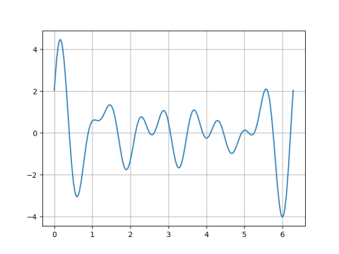
To illustrate this theorem, we’ll look at a couple random trigonometric polynomials with n = 5 and N = 9 and see how many zeros they have. Theory says they should have at least 10 zeros.

The first has 16 zeros:

And the second has 12 zeros:

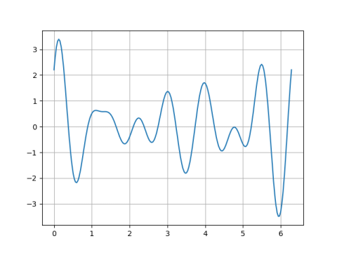
(It’s difficult to see just how many zeros there are in the plots above, but if we zoom in by limiting the vertical axis we can see the zeros more easily. For example, we can see that the second plot does not have a zero between 4 and 5; it almost reaches up to the x-axis but doesn’t quite make it.)

Here’s the code that made these plots.

    import matplotlib.pyplot as plt
    import numpy as np
    
    n = 5
    N = 9
    np.random.seed(20210114)
    
    for p in range(2):
        a = np.random.random(size=N+1)
        b = np.random.random(size=N+1)
    
        x = np.linspace(0, 2*np.pi, 200)
        y = np.zeros_like(x)
        for k in range(n, N+1):
            y += a[k]*np.sin(k*x) + b[k]*np.cos(k*x)
        plt.plot(x, y)
        plt.grid()
        plt.savefig(f"sturm{p}.png")
        plt.ylim([-0.1, 0.1])
        plt.savefig(f"sturm{p}zoom.png")
        plt.close()