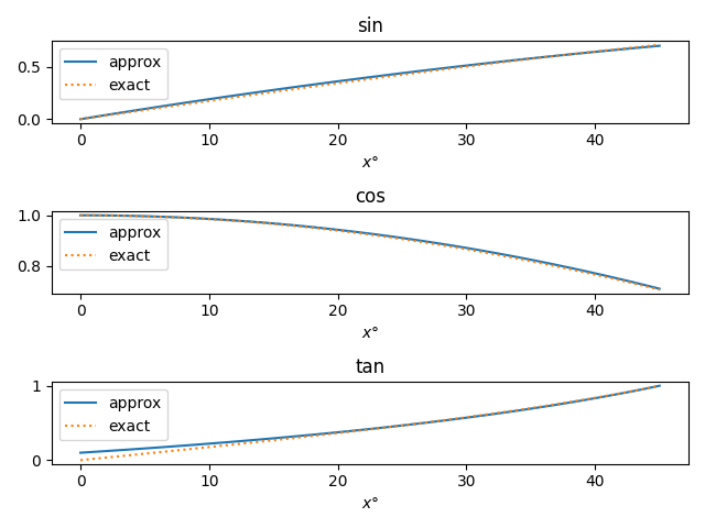
Anthony Robin gives three simple approximations for trig functions in degrees in [1].

The following plots show that these approximations are pretty good. It’s hard to distinguish the approximate and exact curves.
The accuracy of the approximations is easier to see when we subtract off the exact values.
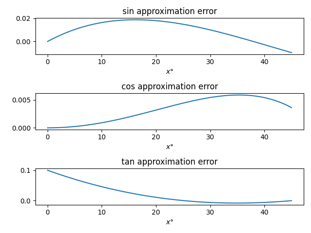
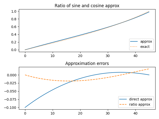
The only problem is that the tangent approximation is poor for small angles [2]. The ratio of the sine and cosine approximations makes a much better approximation, but it this requires more work to evaluate. You could use the ratio for small angles, say less than 20°, and switch over to the tangent approximation for larger angles.
Update: The approximations from this post and several similar posts are all consolidated here.
Here’s the Python code that was used to create the plots in this post. It uses one trick you may find interesting, using the eval function to bridge between the names of functions and the functions themselves.
from numpy import sin, cos, tan, linspace, deg2rad
import matplotlib.pyplot as plt

sin_approx = lambda x: 0.01*x*(2-0.01*x)
cos_approx = lambda x: 1 - x*x/7000.0
tan_approx = lambda x: (10.0 + x)/(100.0 - x)

trig_functions = ["sin", "cos", "tan"];
x = linspace(0, 45, 100)

fig, ax = plt.subplots(3,1)
for n, trig in enumerate(trig_functions):
    ax[n].plot(x, eval(trig + "_approx(x)"))
    ax[n].plot(x, eval(trig + "(deg2rad(x))"), ":")
    ax[n].legend(["approx", "exact"])
    ax[n].set_title(trig)
    ax[n].set_xlabel(r"$x\degree$")

plt.tight_layout()
plt.savefig("trig_approx_plot.png")

fig, ax = plt.subplots(3,1)
for n, trig in enumerate(trig_functions):
    y = eval(trig + "_approx(x)")
    z = eval(trig + "(deg2rad(x))")
    ax[n].plot(x, y-z)
    ax[n].set_title(trig + " approximation error")
    ax[n].set_xlabel(r"$x\degree$")

plt.tight_layout()
plt.savefig("trig_approx_error.png")

tan_approx2 = lambda x: sin_approx(x)/cos_approx(x)

fig, ax = plt.subplots(2, 1)
y = tan(deg2rad(x))
ax[0].plot(x, tan_approx2(x))
ax[0].plot(x, y, ":")
ax[0].legend(["approx", "exact"], loc="lower right")
ax[0].set_title("Ratio of sine and cosine approx")
ax[1].plot(x, y - tan_approx(x), "-")
ax[1].plot(x, y - tan_approx2(x), "--")
ax[1].legend(["direct approx", "ratio approx"])
ax[1].set_title("Approximation errors")

plt.tight_layout()
plt.savefig("tan_approx.png")
Related posts
- Calculating normal probabilities with a simple calculator
- Trig functions across programming languages
[1] Anthony C. Robin. Simple Trigonometric Approximations. The Mathematical Gazette, Vol. 79, No. 485 (Jul., 1995), pp. 385-387
[2] When I first saw this I thought “No big deal. You can just use tan θ ≈ θ for small angles, or tan θ ≈ θ + θ³/3 if you need more accuracy.” But these statements don’t apply here because we’re working in degrees, not radians.
tan θ° is not approximately θ for small angles but rather approximately π θ / 180. If you’re working without a calculator you don’t want to multiply by π if you don’t have to, and a calculator that doesn’t have keys for trig functions may not have a key for π.
Because the cos approximation is more accurate than the sin approximation, you can just shift the cos graph 180 units to the left to get the sin graph, but with higher accuracy.
cos(x) ≈ 1 – (x² / 7000)
so,
sin(x) ≈ 1 – ( (90 – x)² / 7000)
Then you get the same graph, but more accurate than the original sin approximation listed here.
(minor typo edit for my original comment: that sentence should have said “90 units to the right”, not “180 units to the left”. the equations were written correctly though)
This is why the Sinecal Quadrant was invented. Just need to know how to use one.
Thank you sooooooooo much for this. An app I use does not support trig functions, and I’ve been searching for something like this for weeks.
minor typo: Maybe consider “using the eval function to *bridge* between the names of functions and the functions themselves” instead of “using the eval function to between the names of functions and the functions themselves”.