A theorem by Paley and Wiener says that a Fourier series with random coefficients produces Brownian motion on [0, 2π]. Specifically,
![]()
produces Brownian motion on [0, 2π]. Here the Zs are standard normal (Gaussian) random variables.
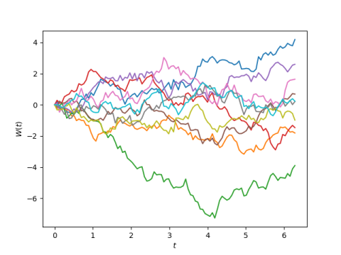
Here is a plot of 10 instances of this process.
Here’s the Python code that produced the plots.
    import matplotlib.pyplot as plt
    import numpy as np

    def W(t, N):
        z = np.random.normal(0, 1, N)
        s = z[0]*t/(2*np.pi)**0.5
        s += sum(np.sin(0.5*n*t)*z[n]/n for n in range(1, N))*2/np.pi**0.5
        return s

    N = 1000
    t = np.linspace(0, 2*np.pi, 100)

    for _ in range(10):
        plt.plot(t, W(t, N))

    plt.xlabel("$t$")
    plt.ylabel("$W(t)$")
    plt.savefig("random_fourier.png")
Note that you must call the function W(t, N) with a vector t of all the time points you want to see. Each call creates a random Fourier series and samples it at the points given in t. If you were to call W with one time point in each call, each call would be sampling a different Fourier series.
The plots look like Brownian motion. Let’s demonstrate that the axioms for Brownian motion are satisfied. In this post I give three axioms as
- W(0) = 0.
- For s > t ≥ 0. W(s) – W(t) has distribution N(0, s – t).
- For v ≥ u ≥ s ≥ t ≥ 0. W(s) – W(t) and W(v) – W(u) are independent.
The first axiom is obviously satisfied.
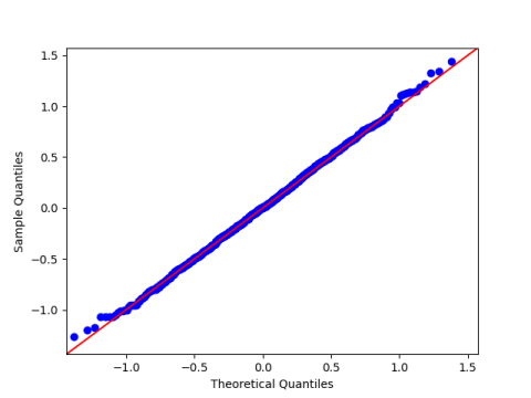
To demonstrate the second axiom, let t = 0.3 and s = 0.5, just to pick two arbitrary points. We expect that if we sample W(s) – W(t) a large number of times, the mean of the samples will be near 0 and the sample variance will be around 0.2. Also, we expect the samples should have a normal distribution, and so a quantile-quantile plot would be nearly a straight 45° line.
To demonstrate the third axiom, let u = 1 and v = √7, two arbitrary points in [0, 2π] larger than the first two points we picked. The correlation between our samples from W(s) – W(t) and our samples from W(v) – W(u) should be small.
First we generate our samples.
    N = 1000
    diff1 = np.zeros(N)
    diff2 = np.zeros(N)
    x = [0.3, 0.5, 1, 7**0.5]
    for n in range(N):
        w = W(x)
        diff1[n] = w[1] - w[0]
        diff2[n] = w[3] - w[2]
Now we test axiom 2.
    from statsmodels.api import qqplot
    from scipy.stats import norm

    print(f"diff1 mean = {diff1.mean()}, var = {diff1.var()}.")
    qqplot(diff1, norm(0, 0.2**0.5), line='45')
    plt.savefig("qqplot.png")
When I ran this the mean was 0.0094 and the variance was 0.2017.
Here’s the Q-Q plot:
And we finish by calculating the correlation between diff1 and diff2. This was 0.0226.
Hi Johan,
A slight change of the code to make it runable:
x = [0.3, 0.5, 1, 7**0.5] => x = np.array([0.3, 0.5, 1, 7**0.5])
w = W(x) => w = W(x, N)
Regards!
Jicun