Monte Carlo integration, or “integration by darts,” is a general method for evaluating high-dimensional integrals. Unfortunately it’s slow. This motivated the search for methods that are like Monte Carlo integration but that converge faster.
Quasi-Monte Carlo (QMC) methods use low discrepancy sequences that explore a space more efficiently than random samples. These sequences are deterministic but in some ways behave like random sequences, hence the name.
On the right problem, QMC integration can be very efficient. On other problems QMC can be mediocre. This post will give an example of each.
Computing ζ(3)
The first example comes from computing the sum
![]()
which equals ζ(3), the Riemann zeta function evaluated at 3.
A few days ago I wrote about ways to compute ζ(3). The most direct way of computing the sum is slow. There are sophisticated ways of computing the sum that are much faster.
There is an integral representation of ζ(3), and so one way to numerically compute ζ(3) would be to numerically compute an integral.
![]()
Let’s see how well quasi-Monte Carlo integration works on this integral. We will use a lattice rule, evaluating our integrand at the points of a quasi-Monte Carlo sequence
![]()
and averaging the results. (Lattice sequences are a special case of quasi-Monte Carlo sequences.)
The notation {x} denotes the fractional part of x. For example, {π} = 0.14159….
Here’s some Python code to compute the integral.
    import numpy as np

    def f(x): return 1/(1 + x[0]*x[1]*x[2])

    v = np.sqrt(np.array([2,3,5]))
    def g(N): return sum( f(n*v % 1) for n in range(1,N+1) ) / N
And here’s a plot that shows how well this does as a function of N.
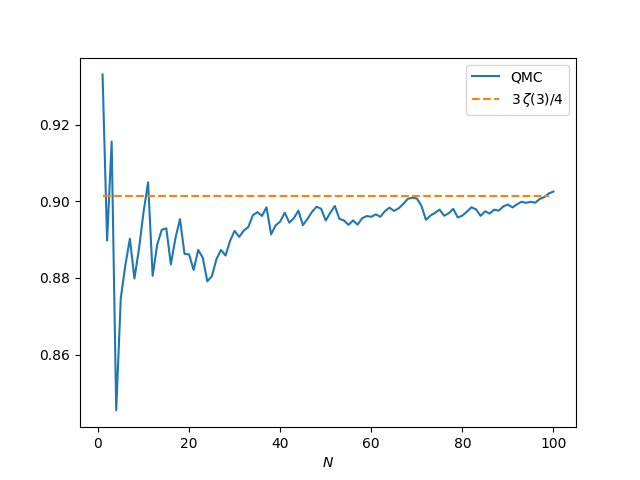
The results are mediocre. The averages are converging to the right value as N increases, but the accuracy isn’t great. When N = 100 the error is 0.001, larger than the error from summing 100 terms of the sum defining ζ(3).
I want to make two points about this example before moving on to the next example.
First, this doesn’t mean that evaluating ζ(3) by computing an integral is necessarily a bad idea; a more efficient integration method might compute ζ(3) fairly efficiently.
Second, this doesn’t mean that QMC is a poor integration method, only that there are better ways to compute this particular integral. QMC is used a lot in practice, especially in financial applications.
Periodic integrands
The lattice rule above works better on periodic integrands. Of course in practice a lot of integrands are not periodic. But if you have an efficient way to evaluate periodic integrands, you can do a change of variables to turn your integration problem into one involving a periodic integrand.
We’ll use the same QMC sequence as above with the integrand
f(x, y, z) = x (1 − x) sin πy
which has integral 1/3π over the unit cube. Here’s a plot of the accuracy as the number of integration points N increases.
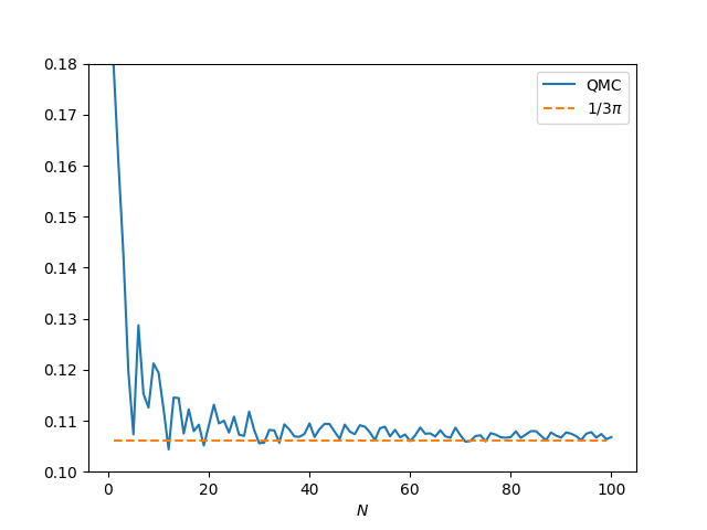
This is much better than before. The error is 0.0007 when N = 100. As N increases, the error goes down more rapidly than with the example above. When computing ζ(3), the error is about 0.001, whether N = 100 or 1,000. In this example, when N = 1,000 the error drops to 0.00003.
This example is periodic in x, y, and z, but the periodic extension is only continuous. The extension has a cusp when x or y take on integer values, and so the derivative doesn’t exist at those points.
If we square our integrand, setting
f(x, y, z) = x² (1 − x)² sin² πy
then the periodic extension is differentiable, and the integration method converges more quickly. The exact integral over the unit cube is 1/60.
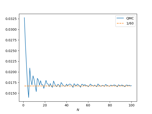
Now our approximation error is about 7.3 ×10⁻⁵ when N = 100, 7.8 ×10⁻⁶ when N = 1,000, and 9.5 ×10⁻⁸ when N = 10,000.
Lattice rules work best on smooth, periodic integrands. If the integrand is smooth but not periodic and you want to use a lattice rule for integration, you’ll get better results if you first do a change of variables to create a smooth, periodic integrand.