Let’s play a game that’s something like Go in three dimensions. Our game is played on the lattice of points in 3D that have integer coordinates. Someone places stones on two lattice points, and your job is to create a path connecting the two stones by adding stones to neighboring locations.
Game cube
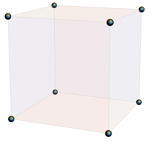
We don’t really have a game “board” since we’re working in three dimensions. We have a game scaffold or game cube. And we can’t just put our stones down. We have to imagine the stones has having hooks that we can use to hang them where pieces of scaffolding come together.
Basic moves
Now for the rules. Our game is based on identities for a function with depending on three parameters: a, b, and c. A location in our game cube is a point with integer coordinates (i, j, k) corresponding to function parameters
(a+i, b+j, c+k).
If there is a stone at (i, j, k) then we are allowed to place stones at neighboring locations if there is a function identity corresponding to these points. The function identities are the “contiguous relations” for hypergeometric functions. You don’t need to know anything about hypergeometric functions to play this game. We’re going to leave out a lot of detail.
Our rule book for identities will be Handbook of Mathematical Function by Abramowitz and Stegun, widely known as A&S. You can find a copy online here.
For example, equation 15.2.10 from A&S relates
F(a, b; c; z)
to
F(a-1, b; c; z)
and
F(a+1, b; c; z).
So if we have a stone at (i, j, k) we can add stones at (i-1, j, k) and (i+1, j, k). Or we could add stones at (i+1, j, k) and (i+2, j, k). You can turn one stone into a row of three stones along the first axis overlapping the original stone.
Equation 15.2.11 lets you do something analogous for incrementing the 2nd coordinate, and Equation 15.2.12 lets you increment the 3rd coordinate. So you could replace a stone with a row of three stones along the second or third axes as well.
This shows that it is always possible to create a path between two lattice points. If you can hop between stones a distance 1 apart, you can create a path that will let you hop between any two points.
Advanced moves
There are other possible steps. For example, equation 15.2.25 has the form
… F(a, b; c; z) + … F(a, b-1; c; z) + … F(a, b; c+1; z) = 0
I’ve left out the coefficients above, denoting them by ellipses. (More on that below.) This identity says you don’t just have to place stones parallel to an axis. For example, you can add a stone one step south and another one step vertically in the same move.
The previous section showed that it’s always possible to create a path between two lattice points. This section implies the finding the shortest path between two points might be a little more interesting.
Applications
There are practical applications to the game described in this post. One reason hypergeometric functions are so useful is that they satisfy a huge number of identities. There are libraries of hypergeometric identities, and there are still new identities to discover and new patterns to discover for organizing the identities.
The moves in the game above can be used to speed up software. Hypergeometric functions are expensive to evaluate, and so it saves time to compute a new function in terms of previously computed functions rather than having to compute it from scratch.
I used this trick to speed up clinical trial simulations. Consecutive steps in the simulation required evaluating contiguous hypergeometric functions, so I could compute one or two expensive functions at the beginning of the simulation and bootstrap them to get the rest of the values I needed.
Coefficients
I’d like to close by saying something about the coefficients in these identities. The coefficients are complicated and don’t have obvious patterns, and so they distract from the underlying structure discussed here. You could stare at a list of identities for a while before realizing that apart from the coefficients the underlying relationships are simple.
All the coefficients in the identities cited above are polynomials in the variables a, b, c, and z. All have degree at most 2, and so they can be computed quickly.
The identities discussed here are often called linear relations. The relations are linear in the hypergeometric functions, but the coefficients are not linear.