Efficiently testing a black box

Suppose you have a black box that takes three bits as input and produces one bit as output. You could think of the input bits as positions of toggle switches, and the output bit as a light attached to the box that is either on or off.

Full factorial design

Now suppose that only one combination of 3 bits produces a successful output. There’s one way to set the switches that makes the light turn on. You can find the successful input by brute force if you test all 2³ = 8 possible inputs. In statistical lingo, you are conducting an experiment with a factorial design, i.e. you test all combinations of inputs.

See the Python code below for a text version of this design

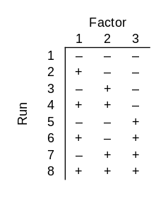
In the chart above, each row is an experimental run and each column is a bit. I used – and + rather than 0 and 1 because it is conventional in this topic to use a minus sign to indicate that a factor is not present and a plus sign to indicate that it is present.

Fractional factorial design

Now suppose your black box takes 4 bits as inputs, but only 3 of them matter. One of the bits does nothing, but you don’t know which bit that is. You could use a factorial design again, testing all 24 = 16 possible inputs. But there’s a more clever approach that requires only 8 guesses. In statistical jargon, this is a fractional factorial design.

See the Python code below for a text version of this design

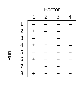
No matter which three bits the output depends on, all combinations of those three bits will be tested. Said another way, if you delete any one of the four columns, the remaining columns contain all combinations of those bits.

Replications

Now suppose your black box takes 8 bits. Again only 3 bits matter, but you don’t know which 3. How many runs do you need to do to be certain of finding the successful combination of 3 bits? It’s clear that you need at least 8 runs: if you know that the first three bits are the important ones, for example, you still need 8 runs. And it’s also clear that you could go back to brute force and try all 28 = 256 possible inputs, but the example above raises your hopes that you could get by with less than 256 runs. Could you still get by with 8? That’s too much to hope for, but you could use only 16 runs.

--------, +----+++, -+--+-++, ++--++--, --+-+++-, +-+-+--+, -++--+-+, +++---+-, ---+++-+, +--++-+-, -+-+-++-, ++-+---+, --++--++, +-++-+--, -++++---, ++++++++

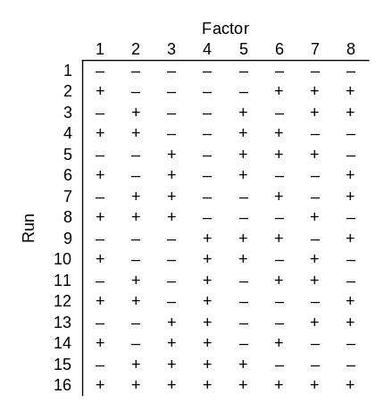
Note that since this design works for 8 factors, it also works for fewer factors. If you had 5, 6, or 7 factors, you could use the first 5, 6, or 7 columns of the design above.

This design has some redundancy: every combination of three particular bits is tested twice. This is unfortunate in our setting because we are assuming the black box is deterministic: the right combination of switches will always turn the light on. But what if the right combination of switches probably turns on the light? Then redundancy is a good thing. If there’s an 80% chance that the right combination will work, then there’s a 96% chance that at least one of the two tests of the right combination will work.

Fractional factorial experiment designs are usually used in with the assumption that there are random effects, and so redundancy is a good thing.

You want to test each main effect, i.e. each single bit, and interaction effects, i.e. combinations of bits, such as pairs of bits or triples of bits. But you assume that not all possible interactions are important; otherwise you’d need a full factorial design. You typically hit diminishing return with interactions quickly: pairs of effects are often important, combinations of three effects are less common, and rarely would an experiment consider forth order interactions.

If only main effects and pairs of main effects matter, and you have a moderately large number of factors n, a fractional factorial design can let you use a lot less than 2n runs while giving you as many replications of main and interaction effects as you want.

Verification

The following Python code verifies that the designs above have the claimed properties.

    import numpy as np
    from itertools import combinations
    
    def verify(matrix, k):
        "verify that ever choice of k columns has 2^k unique rows"
        nrows, ncols = matrix.shape
        for (a, b, c) in combinations(range(ncols), k):
            s = set()
            for r in range(nrows):
                s.add((matrix[r,a], matrix[r,b], matrix[r,c]))
            if len(s) != 2**k:
                print("problem with columns", a, b, c)
                print("number of unique elements: ", len(s))
                print("should be", 2**k)
                return
        print("pass")
    
    m = [
        [-1, -1, -1, -1],
        [-1, -1, +1, +1],
        [-1, +1, -1, +1],
        [-1, +1, +1, -1],
        [+1, -1, -1, +1],
        [+1, -1, +1, -1],
        [+1, +1, -1, -1],
        [+1, +1, +1, +1]
    ]
    
    verify(np.matrix(m), 3)
    
    m = [
        [-1, -1, -1, -1, -1, -1, -1, -1],
        [+1, -1, -1, -1, -1, +1, +1, +1],
        [-1, +1, -1, -1, +1, -1, +1, +1],
        [+1, +1, -1, -1, +1, +1, -1, -1],
        [-1, -1, +1, -1, +1, +1, +1, -1],
        [+1, -1, +1, -1, +1, -1, -1, +1],
        [-1, +1, +1, -1, -1, +1, -1, +1],
        [+1, +1, +1, -1, -1, -1, +1, -1],
        [-1, -1, -1, +1, +1, +1, -1, +1],
        [+1, -1, -1, +1, +1, -1, +1, -1],
        [-1, +1, -1, +1, -1, +1, +1, -1],
        [+1, +1, -1, +1, -1, -1, -1, +1],
        [-1, -1, +1, +1, -1, -1, +1, +1],
        [+1, -1, +1, +1, -1, +1, -1, -1],
        [-1, +1, +1, +1, +1, -1, -1, -1],
        [+1, +1, +1, +1, +1, +1, +1, +1],
    ]
    
    verify(np.matrix(m), 3)

Related services

The original Room square

A few days ago I wrote about Room squares, squares named after Thomas Room. This post will be about Room’s original square.

You could think of a Room square as a tournament design in which the rows represent locations and the columns represent rounds (or vice versa). Every team plays every other team exactly once, and only one pair of teams can play each other at the same location in the same round.

Here is an image creating from Room’s original square using the visualization approach from the earlier post.

This is not a trivial variation on the square in the earlier post. Notice that this square has a block of four contiguous squares in the middle row and middle column. The previous image does not.

Here is Room’s original square, presented as in his half-page announcement in [1] with the rows and columns labeled with binary numbers.

A plain text version of the image above is available below [2].

Room points out an interesting pattern: a cell is filled in if and only if the “dot product” of its coordinate is odd. Think of each coordinate number as three dimensional vector and take the dot product of the vector representing the row and the vector representing the column.

Room didn’t refer to dot products. In his words

(αβγ, λμν) are the coordinates of one of the points marked rs in and only if αλ + βμ + γν is odd.

Related posts

[1] T. G. Room. A new type of magic square. Mathematical Gazette. Volume 39 (1955), p. 307.

[2] Here is Room’s square as a plain text (org-mode) table.

|-----+-----+-----+-----+-----+-----+-----+-----|
| 001 |  12 |     |  34 |     |  56 |     |  78 |
| 010 |     |  37 |  25 |     |     |  48 |  16 |
| 011 |  47 |  15 |     |     |  38 |  26 |     |
| 100 |     |     |     |  68 |  14 |  57 |  23 |
| 101 |  58 |     |  67 |  24 |     |  13 |     |
| 110 |     |  46 |  18 |  35 |  27 |     |     |
| 111 |  36 |  28 |     |  17 |     |     |  45 |
|-----+-----+-----+-----+-----+-----+-----+-----|
|     | 001 | 010 | 011 | 100 | 101 | 110 | 111 |
|-----+-----+-----+-----+-----+-----+-----+-----|

Room squares and Tournaments

A Room square is a variation on a Latin square. Room squares are named after Thomas Room, though there is an application to rooms as in compartments of a building that we’ll discuss below.

In a Latin square of size n you have to assign one of n symbols to each cell so that each symbol appears exactly once in each row and column. A Room square is sort of a Latin square with pairs.

Each cell of a Room square is either empty or contains an unordered pair of symbols. Each symbol appears exactly once in each row and column, and every possible pair of symbols appears in some cell.

The following graphic shows a 7 × 7 Room square with eight symbols, each represented by a different color.

If you have trouble seeing some of the colors, take a look at the code below that made the image.

An n × n Room square corresponds to a Round Robin tournament schedule with n + 1 players. Each row represents a location (or room), and each column represents a round. Each player plays one game in each round, and each pair of players plays in exactly one location.

Python code

Here’s the code I wrote to create the image above.

    import matplotlib.pyplot as plt
    
    colors = ["red", "orange", "yellow", "green", "blue", "black", "gray", "purple"]
    up, dn = True, False
    
    def draw_triangle(row, col, value, pos):
        if pos == up:
            x = [col, col, col+1]
            y = [row, row+1, row+1]
        else:
            x = [col, col+1, col+1]
            y = [row, row, row+1]
        plt.fill(x, y, colors[value])
    
    sq = [
        (1, 3, 0, 4),
        (1, 5, 3, 5),
        (1, 6, 1, 2),
        (1, 7, 7, 6),
        (2, 2, 6, 3),
        (2, 4, 2, 4),
        (2, 5, 0, 1),
        (2, 6, 7, 5),
        (3, 1, 5, 2),
        (3, 3, 1, 3),
        (3, 4, 6, 0),
        (3, 5, 7, 4),
        (4, 2, 0, 2),
        (4, 3, 5, 6),
        (4, 4, 7, 3),
        (4, 7, 4, 1),
        (5, 1, 6, 1),
        (5, 2, 4, 5),
        (5, 3, 7, 2),
        (5, 6, 3, 0),
        (6, 1, 3, 4),
        (6, 2, 7, 1),
        (6, 5, 2, 6),
        (6, 7, 5, 0),
        (7, 1, 7, 0),
        (7, 4, 1, 5),
        (7, 6, 4, 6),
        (7, 7, 2, 3)
    ]
        
    for t in sq:
        draw_triangle(t[0], t[1], t[2], up)
        draw_triangle(t[0], t[1], t[3], dn)    
    plt.grid()
        
    plt.gca().set_aspect("equal")
    plt.show()

Related posts

Costas arrays in Mathematica

A couple days ago I wrote about Costas arrays. In a nutshell, a Costas array of size n is a solution to the n rooks problem, with the added constraint that if you added wires between the rooks, no two wires would have the same length and slope. See the earlier post for more details.

The earlier post implemented the Lempel algorithm in Python. Here we’ll implement it in Mathematica. Lempel’s algorithm says to start with parameters p and a where p is a prime and a is a primitive root mod p [1]. Then you can create a Costas array of size n = p-2 by filling in the (i, j) square if and only if

ai + aj = 1 mod p.

We can implement this in Mathematica by

    fill[i_, j_, p_, a_] := If[Mod[a^i + a^j, p] == 1, 1, 0]
    m[p_, a_] := Table[fill[i, j, p, a], {i, 1, p - 2}, {j, 1, p - 2}]

We could visualize the Costas array generated by p = 11 and a = 2 using ArrayPlot. The code

    ArrayPlot[m[11, 2], Mesh -> All]

Generates the following image.

Note that the image is symmetric with respect to the main diagonal. That’s because our algorithm is symmetric in i and j. But Costas arrays are not always symmetrical, so this underscores the point that there is no known scalable algorithm for finding all Costas arrays.

In this example we started with knowing that 2 was a primitive root mod 11. We could have had Mathematica pick a primitive root mod p for us by calling PrimitiveRoot[p]

Just out of curiosity, let’s redo the example above, but instead of testing whether

ai + aj = 1 mod p.

we’ll just use ai + aj mod p.

The code

    ArrayPlot[Table[Mod[2^i + 2^j, 11], {i, 1, 9}, {j, 1, 9}]]

produces the following image.

[1] Lempel’s algorithm generalizes to finite fields of any order, not just integers modulo a prime.

Costas arrays

The famous n queens problem is to find a way to position n queens on a n×n chessboard so that no queen attacks any other. That is, no two queens can be in the same row, the same column, or on the same diagonal. Here’s an example solution:

Costas arrays

In this post we’re going to look at a similar problem, weakening one requirement and adding another. First we’re going to remove the requirement that no two pieces can be on the same diagonal. This turns the n queens problem into the n rooks problem because rooks cannot move diagonally.

Next, imagine running stiff wires from every rook to every other rook. We will require that no two wires have the same length and run in the same direction. in more mathematical terms, we require that the displacement vectors between all the rooks are unique.

A solution to this problem is called a Costas array.  In 1965, J. P. Costas invented what are now called Costas arrays to solve a problem in radar signal processing.

Why do we call a solution a Costas array rather than a Costas matrix? Because a matrix solution can be described by recording for each column the row number of the occupied cell. For example, we could describe the eight queens solution above as

(2, 4, 6, 8, 3, 1, 7, 5).

Here I’m numbering rows from the bottom up, like points in the first quadrant, rather than top to bottom as one does with matrices.

Note that the solution to the eight queens problem above is not a Costas array because some of the displacement vectors between queens are the same. For example, if we number queens from left to right, the displacement vectors between the first and second queens is the same as the displacement vector between the second and third queens.

Visualizing a Costas array

Here’s a visualization of a Costas array of order 5.

It’s clear from the plot that no two dots are in the same row or column, but it’s not obvious that all the connecting lines are different. To see that the lines are different, we move all the tails of the connecting lines to the origin, keeping their length and direction the same.

There are 10 colored lines in the first plot, but at first you may only see 9 in the second plot. That’s because two of the lines have the same direction but different length. If you look closely, you’ll see that there’s a short purple line on top of the long red line. That is, one line runs from the origin to (1, -1) and another from the origin to (4, -4).

Here is a visualization of a Costas array of order 9.

And here are its displacement vectors translated to the origin.

Here is a visualization of a Costas array of order 15.

And here are its displacement vectors translated to the origin.

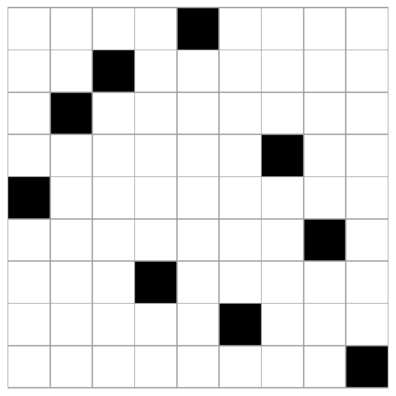
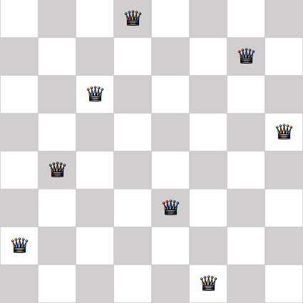
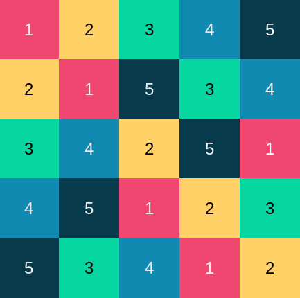
Generating Costas arrays

There are algorithms for generating some Costas arrays, but not all. Every known algorithm [1] leaves out some solutions, and it is not know whether Costas arrays exist for some values of n.

The Costas arrays above were generated using the Lempel construction algorithm. Given a prime p [2] and a primitive root mod p [3], the following Python code will generate a Costas array of order p – 2.


    p = 11 # prime
    a = 2 # primitive element

    # verify a is a primitive element mod p
    s = {a**i % p for i in range(p)}
    assert( len(s) == p-1 )

    n = p-2
    dots = []

    for i in range(1, n+1):
        for j in range(1, n+1):
            if (pow(a, i, p) + pow(a, j, p)) % p == 1:
                dots.append((i,j))
                break

Related posts

[1] Strictly speaking, no scalable algorithm will enumerate all Costas arrays. You could enumerate all permutation matrices of order n and test whether each is a Costas array, but this requires generating and testing n! matrices and so is completely impractical for moderately large n.

[2] More generally, the Lempel algorithm can generate a solution of order q-2 where q is a prime power. The code above only works for primes, not prime powers. For prime powers, you have to work with finite fields of order q and the code would be more complicated.

[3] A primitive root for a finite field of order q is a generator of the multiplicative group of the field, i.e. an element x such that every non-zero element of the field is some power of x.

Balanced tournament designs

Suppose you have an even number of teams that you’d like to schedule in a Round Robin tournament. This means each team plays every other team exactly once.

Denote the number of teams as 2n. You’d like each team to play in each round, so you need n locations for the games to be played.

Each game will choose 2 teams from the set of 2n teams, so the number of games will be n(2n – 1). And this means you’ll need 2n – 1 rounds. A tournament design will be a grid with n rows, one for each location, and 2n-1 columns, one for each round.

Let’s pause there for just a second and make sure this is possible. We can certainly assign n(2n – 1) games to a grid of size n by 2n-1. But can we do it in such a way that no team needs to be in two locations at the same time? It turns out we can.

Now we’d like to introduce one more requirement: we’d like to balance the games over the locations. By that we mean we’d like a team to play no more than twice in the same location. A team has to play at least once in each location, but not every team can play twice in each location. If every team played once in each location, we’d have n² games, and if every team played twice in each location we’d have 2n² games, but

n² < n(2n – 1) < 2n²

for n greater than 1. If n = 1, this is all trivial, because in that case we would have two teams. They simply play each other and that’s the tournament!

We can’t have each team play exactly the same number of times in each location, but can we have each team play either once or twice in each location? If so, we call that a balanced tournament design.

Now the question becomes for which values of n can we have a balanced tournament design involving 2n teams. This is called a BTD(n) design.

We said above that this is possible if n = 1: two teams just play each other somewhere. For n = 2, it is not possible to have a balanced tournament design: some team will have to play all three games in the same location.

It is possible to have a balanced tournament design for n = 3. Here’s a solution:

{{af, ce, bc, de, bd}, {be, df, ad, ac, cf}, {cd, ab, ef, bf, ae}}

In fact this is the solution aside from relabeling the teams. That is, given any balanced tournament design involving six teams, there is a way to label the teams so that you have the design above. Said another way, there is one design in BTD(3) up to isomorphism.

There are balanced tournament designs for all positive n except for n = 2. And in general there are a lot of them. There are 47 designs in BTD(4) up to isomorphism [1].

Related posts

[1] The CRC Handbook of Combinatorial Designs. Colbourn and Dinitz editors. CRC Press, 1996.


Self-Orthogonal Latin Squares

The other day I wrote about orthogonal Latin squares. Two Latin squares are orthogonal if the list of pairs of corresponding elements in the two squares contains no repeats.

A self-orthogonal Latin square (SOLS) is a Latin square that is orthogonal to its transpose.

Here’s an example of a self-orthogonal Latin square:

    1 7 6 5 4 3 2
    3 2 1 7 6 5 4
    5 4 3 2 1 7 6
    7 6 5 4 3 2 1
    2 1 7 6 5 4 3
    4 3 2 1 7 6 5
    6 5 4 3 2 1 7

To see that this Latin square is orthogonal to itself, we’ll concatenate the square and its transpose.

    11 73 65 57 42 34 26 
    37 22 14 76 61 53 45 
    56 41 33 25 17 72 64 
    75 67 52 44 36 21 13 
    24 16 71 63 55 47 32 
    43 35 27 12 74 66 51 
    62 54 46 31 23 15 77

Each pair of digits is unique.

Magic squares

As we discussed in the earlier post, you can make a magic square out of a pair of orthogonal Latin squares. If we interpret the pairs of digits above as base 10 numbers, we have a magic square because each row, column, and diagonal has the digits 1 through 7 in the 1s place and the same set of digits in the 10s place.

Typically an n × n magic square is filled with the numbers 1 through n². We can make such a magic square with a few adjustments.

First, we subtract 1 from every element of our original square before we combine it with its transpose. This gives us the following.

    00 62 54 46 31 23 15 
    26 11 03 65 50 42 34 
    45 30 22 14 06 61 53 
    64 56 41 33 25 10 02 
    13 05 60 52 44 36 21 
    32 24 16 01 63 55 40 
    51 43 35 20 12 04 66 

If we interpret the elements above as base 7 numbers, then the entries are the numbers 0 through 66seven which equals 48ten. If we add 1 to every entry we get all the numbers from 1 through 100seven = 49ten. Written in base 10, this is the following.

     1 45 40 35 23 18 13 
    21  9  4 48 36 31 26 
    34 22 17 12  7 44 39 
    47 42 30 25 20  8  3 
    11  6 43 38 33 28 16 
    24 19 14  2 46 41 29 
    37 32 27 15 10  5 49 

Possible sizes

It’s surprising that orthogonal Latin squares exist as often as they do. Self-orthogonal Latin squares are more rare, and yet they exist for all sizes except n = 2, 3, or 6. (Source: The CRC Handbook of Combinatorial Designs.)

It’s hard to prove that self-orthogonal Latin squares exist, but it’s easy to verify the sizes where they don’t exist. There is no self-orthogonal Latin square of size 6 because there is no pair of orthogonal Latin squares of size 6. The latter is a hard theorem to prove, but given it, the former is trivial.

There are orthogonal Latin squares of size 3, but no self-orthogonal Latin squares of size 3. And it’s not hard to see why. Suppose there were such a square. Without loss of generality we can label the top row with 1, 2, and 3. Let x be the entry directly below 1.

    1 2 3
    x * *
    * * *

What could x be? Not 1, because elements in a column of a Latin square are unique. It can’t be 2 either, because otherwise when you join the square and its transpose would have two 22s. So x must be 3, and the element below x must be 2. But then when you join the square and its transpose you have two 32s. There’s not enough wiggle room for a 3 × 3 Latin square to be self-orthogonal.

Greco-Latin squares and magic squares

Suppose you create an n × n Latin square filled with the first n letters of the Roman alphabet. This means that each letter appears exactly once in each row and in each column.

You could repeat the same exercise only using the Greek alphabet.

Is it possible to find two n × n Latin squares, one filled with Roman letters and the other filled with Greek letters, so that when you combine corresponding entries, each combination of Roman and Greek letters appears exactly once? If so, the combination is called a Greco-Latin square.

Whether Greco-Latin squares of size n exist depends on n. But before we explore that, let’s give an example.

Here are two Latin squares, one filled with the first four Roman letters and the other filled with the first four Greek letters.

    A B C D   α β γ δ
    D C B A   γ δ α β
    B A D C   δ γ β α
    C D A B   β α δ γ

If we concatenate the two matrices, we get

    Aα Bβ Cγ Dδ   
    Dγ Cδ Bα Aβ   
    Bδ Aγ Dβ Cα   
    Cβ Dα Aδ Bγ   

and each of the two-letter entries is unique. So we’ve shown that a Greco-Latin square exists for n = 4.

Mutually Orthogonal Latin Squares (MOLS)

The more modern name for Greco-Latin squares is “mutually orthogonal Latin squares,” abbreviated MOLS. We say two Latin squares M and N are mutually orthogonal if the list of pairs (Mij, Nij,) contains no duplicates.

Euler’s work

Euler showed how to construct Greco-Latin squares when n is odd and when n is a multiple of 4. He conjectured that no Greco-Latin squares exist when n = 4k + 2.

His conjecture was incorrect. For example, there is a Greco-Latin square of size 10. And in fact, Greco-Latin squares exist for all n except n = 2 and n = 6.

Magic squares

Suppose you have two orthogonal Latin squares M and N of size n, and suppose that the diagonal elements of both squares contain no duplicates.

Use the numbers 0 through n-1 rather than Greek or Latin letters to fill the squares and interpret the Latin squares as matrices. Then the matrix

nM + N

is a magic square. This is equivalent to taking the corresponding Greco-Latin square and interpreting the entries as base n numbers.

For example, using the Latin squares above, replace A and α with 0, B and β with 1, C and γ with 2, and D and γ with 3. Then the Greco-Roman square

    Aα Bβ Cγ Dδ   
    Dγ Cδ Bα Aβ   
    Bδ Aγ Dβ Cα   
    Cβ Dα Aδ Bγ   

becomes

    00 11 22 33   
    32 23 10 01   
    13 02 31 20   
    21 30 03 12   

with the entries being base 4 numbers. The rows and columns clearly have the same sum because they all have the same set of numbers in the 1s place and in the 4s place. Written in base 10, the magic square above is

     0  5 10 15   
    14 11  4  1   
     7  2 13  8   
     9 12  3  6   

It’s conventional for magic squares to be filled with consecutive numbers starting with 1, so you could add 1 to every entry above if you’d like.

Related posts

Latin squares and 3D chess

In a n×n Latin square, each of the numbers 1 through n appears exactly once in each row and column. For example, the 5 × 5 square below is a Latin square.

12345, 21534, 34251, 45123, 53412

If we placed a rook on each square numbered 1, the rooks would not attack each other since no two rooks would be in the same row or the same column. The same would be true if we moved all the rooks to squares numbered 2, or 3, etc.

Now imagine a n×n×n chess cube, a stack of n chessboards, each board being n×n. For example, we could have a stack of eight standard 8×8 boards.

In our 3D chess cube, rooks can move any number of squares in either the x or y direction within a board, and they can also move vertically in the z direction.

Put a rook on every square of the bottom board. Then take the rooks on squares numbered 2 and move them to the second level. Take the rooks on squares numbered 3 and move them to the third level, and so forth.

Now we have n×n rooks, and none is in a position to attack the other. To see this, pick a particular level k. None of the rooks on level k are attacking each other because level k is a Latin square. And none of the rooks can attack vertically because we started with all the rooks on the bottom level and lifted them up by various amounts; there’s only one rook in each vertical column.

Next let’s suppose we have n×n rooks arranged in 3D so that none is attacking any of the others. Label the rooks on level k with a k. Now push all the rooks straight down vertically to the first level. There can only be one rook on each square because no rooks were attacking each other vertically.

Number each square by the number of its rook. I claim the result is a Latin square. There can only be one k in each row and column because all the ks started out on level k, and none were attacking each other in the x or y direction.

Related posts

Aesthetic uses of Latin squares

We think they like randomness in design, but we don’t exactly. People like things that are sorta random, but not too random. When you literally scatter things randomly, they looked too clumped [1].

There are many ways around this problem, variations on randomness that people find more aesthetically pleasing. One of these ways is random Latin squares.

A Latin square of size n is an n × n grid filled with n different things—numbers, letters, colors, etc.— such that each kind of thing appears exactly once in each row and in each column. For example, 26 × 26 grid filled with the letters of the English alphabet is a Latin square if every row and every column contains the entire alphabet; no letters repeated and no letters missing.

A random Latin square is an arrangement that is random but subject to the constraint that it be a Latin square. Random Latin squares look nice because they’re somewhat random but they avoid certain kinds of repetition.

Suppose you have five different colors of tile and you need to lay down the tiles in a 10 × 20 grid. You want to lay down the tiles “randomly” but you don’t want too many of any one color to appear in a small area.

One way to do this would be to divide the 10 × 20 space into a grid of grids. Each subgrid is a 5 × 5 Latin square. Here’s an example.

The image above is a 2 × 4 grid of 5 × 5 grids, and each of the 5 × 5 grids is a Latin square chosen at random.

Here’s another example with five different colors and different random Latin squares.

If you look carefully, you’ll spot a few places where tiles of the same color touch on an edge. This cannot happen within a Latin square, but it can happen where two different Latin squares are next to each other. So the randomization scheme described here allows for a few tiles of the same color to touch but not many.

I expect randomized Latin squares are used this way fairly often. You’d never know, and that’s kinda the point. Someone would have to stare at a pattern like this a long time before they realized that horizontal or vertical segments of five do not repeat a color.

Related posts

[1] One way to detect fraud is to look for fake randomness. When people try to make something look random, they usually fail and leave statistically detectable fingerprints.