A few years ago I wrote several posts about “squircles”, starting with this post. These are shapes satisfying

where typically p = 4 or 5. The advantage of a squircle over a square with rounded edges is that the curvature varies continuously around the figure rather than jumping from a constant positive value to zero.
Manuel Fernández-Guasti developed a slightly different shape also called a squircle but with a different equation

We need to give separate names to the two things called squircles, and so I’ll name them after their parameters: p-squircles and s-squircles.
As s varies from 0 to 1, s-squircles change continuously from a circle to a square, just as p-squircles varies do as p goes from 2 to ∞.
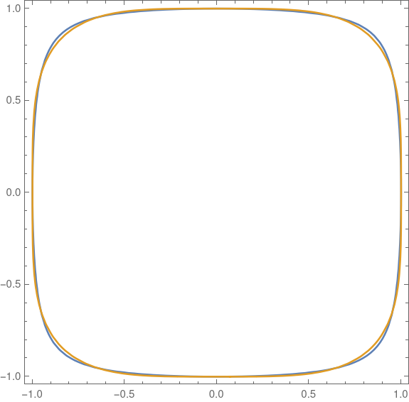
The two kinds of squircles are very similar. Here’s a plot of one on top of the other. I’ll go into detail later of how this plot was made.
Advantage of s-squircles
The equation for a p-squircle is polynomial if p is an even integer, but in general the equation is transcendental. The equation for an s-squircle is a polynomial of degree 4 for all values of s. It’s more mathematically convenient, and more computationally efficient, to have real numbers as coefficients than as exponents. The s-squircle is an algebraic variety, the level set of a polynomial, and so can be studied via algebraic geometry whereas p-squircles cannot (unless p is an even integer).
It’s remarkable that the two kinds of squircles are so different in the structure of their defining equation and yet so quantitatively close together.
Equal area comparison
I wanted to compare the two shapes, so I plotted p-squircles and s-squircles of the same area.
The area of a p-squircle is given here where n = 2. The area of an s-squircle is given here MathWorld where k = 1.

Here E is the “elliptic integral of the second kind.” This function has come up several times on the blog, for example here.
Both area function are increasing functions of their parameters. We have A1(2) = A2(0) and A1(∞) = A2(1). So we can pick a value of p and solve for the corresponding value of s that gives the same area, or vice versa.
The function A1 can be implemented in Mathematica as
A1[p_] := 4 Gamma[1 + 1/p]^2/Gamma[1 + 2/p]
The function A2 is little trickier because Mathematica parameterizes the elliptic integral slightly differently than does the equation above.
A2[s_] := 4 EllipticE[ArcSin[s], s^-2]/s
Now I can solve for the values of s that give the same area as p = 4 and p = 5.
FindRoot[A2[s] == A1[4], {s, 0.9}]
returns 0.927713 and
FindRoot[A2[s] == A1[5], {s, 0.9}]
returns 0.960333. (The 0.9 argument in the commands above is an initial guess at the root.)
The command
    ContourPlot[{x^2 + y^2 == 0.927713 ^2 x^2 y^2 + 1,
        x^4 + y^4 == 1}, {x, -1, 1}, {y, -1, 1}]
produces the following plot. This is the same plot as at the top of the post, but enlarged to show detail.
The command
    ContourPlot[{x^2 + y^2 == 0.960333 ^2 x^2 y^2 + 1,
        Abs[x]^5 + Abs[y]^5 == 1}, {x, -1, 1}, {y, -1, 1}]
produces this plot
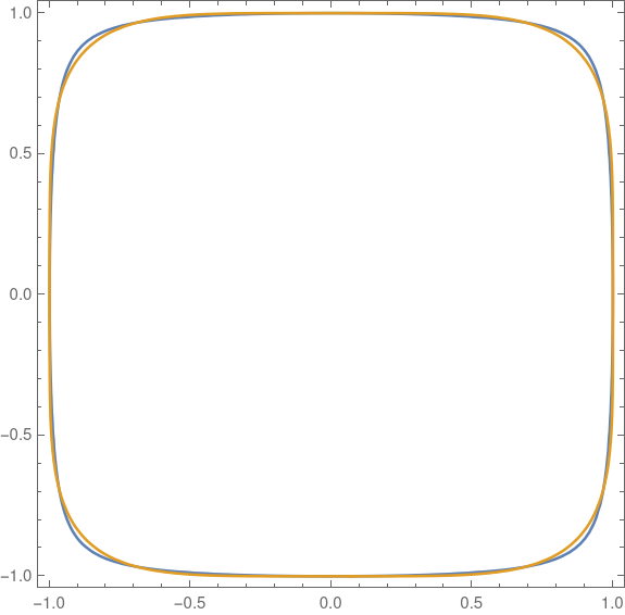
In both cases the s-squircle is plotted in blue, and the p-squircle in gold. The gold virtually overwrites the blue. You have to look carefully to see a little bit of blue sticking out in the corners. The two squircles are essentially the same to within the thickness of the plotting lines.
History
The term “squircle” goes back to 1953, but was first used as it is used here around 1966. More on this here.
However, Fernández-Guasti was the first to use the term in scholarly literature in 2005. See the discussion in the MathWorld article.
A squircle blog post elaborating on a high school math lesson I developed and presented in 2018:
https://bobtechnits.blogspot.com/2018/03/playing-with-equation-for-circle.html
My goal was to nudge the students away from using “math hammers” to solve low-order polynomials (and pass the tests!), to *also* have fun playing with the math itself just to see what happens, then looking for real-world applications.
The students were not impressed with my presentation, though they fortunately engaged better with the blog post.