Here are three curves that have interesting names and interesting shapes.
The fish curve
The fish curve has parameterization
x(t) = cos(t) – sin²(t)/√2
y(t) = cos(t) sin(t)
We can plot this curve in Mathematica with
    ParametricPlot[
        {Cos[t] - Sin[t]^2/Sqrt[2], Cos[t] Sin[t]},
        {t, 0, 2 Pi}]
to get the following.
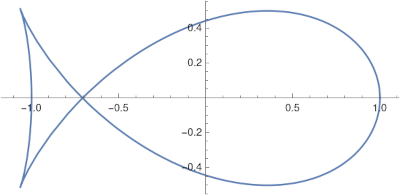
It’s interesting that the image has two sharp cusps: the parameterization consists of two smooth functions, but the resulting image is not smooth. That’s because the velocity of the curve is zero at 3π/4 and 7π/4.
I found the fish curve by poking around Mathematica’s PlainCurveData function. I found the next two in the book Mathematical Models by H. Martyn Cundy and A. P. Rollett.
The electric motor curve
Next is the “electric motor” curve. Cundy and Rollett’s book doesn’t provide illustrations for the plane curves it lists on pages 71 and 72, and I plotted the electric motor curve because I was curious why it was called that.
The curve has equation
y²(y² − 96) = x² (x² − 100)
and we can plot it in Mathematica with
    ContourPlot[ y^2 (y^2 - 96) == x^2 (x^2 - 100),
        {x, -20, 20}, {y, -20, 20}
which gives the following.
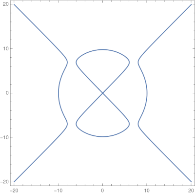
Sure enough, it looks like the inside of an electric motor!
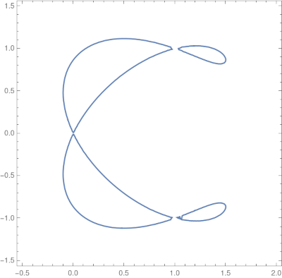
The ampersand curve
I was also curious about the “ampersand curve” because of its name. The curve has equation
(y² − x²) (x − 1) (2x − 3) = 4 (x² + y² − 2x)²
and can be plotted in Mathematica with
    ContourPlot[(y^2 - x^2) (x - 1) (2 x - 3) ==
                 4 (x^2 + y^2 - 2 x)^2,
                 {x, -0.5, 2}, {y, -1.5, 1.5},
                 PlotPoints -> 100]
The produces the following pleasant image.
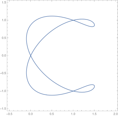
Note that the code specifies PlotPoints. Without this argument, the default plotting resolution produces a misleading plot, making it appear that the curve has three components.