Circulant matrices, eigenvectors, and the FFT

A circulant matrix is a square matrix in which each row is a rotation of the previous row. This post will illustrate a connection between circulant matrices and the FFT (Fast Fourier Transform).

Circulant matrices

Color in the first row however you want. Then move the last element to the front to make the next row. Repeat this process until the matrix is full.

The NumPy function roll will do this rotation for us. Its first argument is the row to rotate, and the second argument is the number of rotations to do. So the following Python code generates a random circulant matrix of size N.

    import numpy as np

    np.random.seed(20230512)
    N = 5
    row = np.random.random(N)
    M = np.array([np.roll(row, i) for i in range(N)])

Here’s the matrix M with entries truncated to 3 decimal places to make it easier to read.

    [[0.556 0.440 0.083 0.460 0.909]
     [0.909 0.556 0.440 0.083 0.460]
     [0.460 0.909 0.556 0.440 0.083]
     [0.083 0.460 0.909 0.556 0.440]
     [0.440 0.083 0.460 0.909 0.556]]    

Fast Fourier Transform

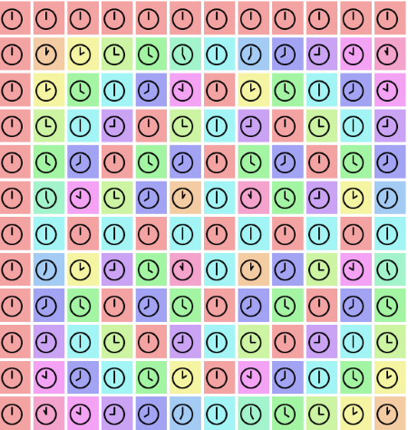
The Fast Fourier Transform is a linear transformation and so it can be represented by a matrix [1]. This the N by N matrix whose (j, k) entry is ω^jk where ω = exp(-2πi/N), with j and k running from 0 to N – 1. [2]

Each element of the FFT matrix corresponds to a rotation, so you could visualize the matrix using clocks in each entry or by a cycle of colors. A few years ago I created a visualization using both clock faces and colors:

Eigenvectors and Python code

Here’s a surprising property of circulant matrices: the eigenvectors of a circulant matrix depend only on the size of the matrix, not on the elements of the matrix. Furthermore, these eigenvectors are the columns of the FFT matrix. The eigenvalues depend on the matrix entries, but the eigenvectors do not.

Said another way, when you multiply a circulant matrix by a column of the FFT matrix of the same size, this column will be stretched but not rotated. The amount of stretching depends on the particular circulant matrix.

Here is Python code to illustrate this.

    for i in range(N):
        ω = np.exp(-2j*np.pi/N)
        col1 = np.array([ω**(i*j) for j in range(N)])
        col2 = np.matmul(M, col1)
        print(col1/col2)

In this code col1 is a column of the FFT matrix, and col2 is the image of the column when multiplied by the circulant matrix M. The print statement shows that the ratios of each elements are the same in each position. This ratio is the eigenvalue associated with each eigenvector. If you were to generate a new random circulant matrix, the ratios would change, but the input and output vectors would still be proportional.

Notes

[1] Technically this is the discrete Fourier transform (DFT). The FFT is an algorithm for computing the DFT. Because the DFT is always computed using the FFT, the transformation itself is usually referred to as the FFT.

[2] Conventions vary, so you may see the FFT matrix written differently.