Kepler triangle

A Kepler triangle is a right triangle whose sides are in geometric progression. That is, if the sides have length a < b < c, then b/a = c/b = k.

All Kepler triangles are similar because the proportionality constant k can only take on one value. To see this, we first pick our units so that a = 1. Then b = k and c = k². By the Pythagorean theorem

a² + b² = c²

and so

1 + k² = k⁴

which means k² equals the golden ratio φ.

Here’s a nice geometric property of the Kepler triangle proved in [1].

Go around the triangle counterclockwise placing a point on each side dividing the side into pieces that are in golden proportion. Connect these three points with the opposite vertex. Then the triangle formed by the intersections of these line segments is also a Kepler triangle.

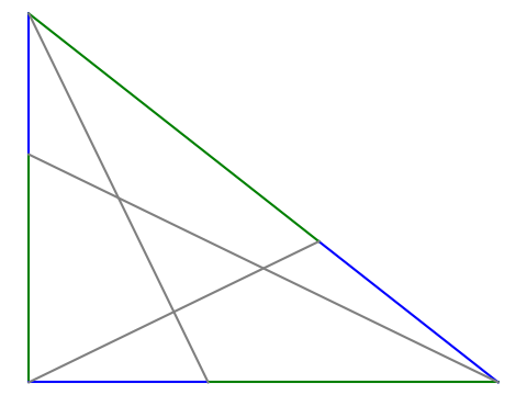
On each side, the ratio of the length of the green segment to the blue segment is φ. The grey triangle in the middle is another Kepler triangle.

The rest of this post will present the code that was used to create the image above.

We’ll need the following imports.

import matplotlib.pyplot as plt
from numpy import array
from numpy.linalg import solve

We’ll also need to define the golden ratio, a function to split a line segment into golden proportions, and a function to draw a line between two points.

φ = (1 + 5**0.5)/2

def golden_split(pt1, pt2):
    return (1/φ)*pt1 + (1 - 1/φ)*pt2

def connect(pt1, pt2, style):
    plt.plot([pt1[0], pt2[0]], [pt1[1], pt2[1]], style)

Now we can draw the figure.

A = array([0, 1])
B = array([0, 0])
C = array([φ**0.5, 0])

X = golden_split(A, B)
Y = golden_split(B, C)
Z = golden_split(C, A)

connect(A, X, "b")
connect(X, B, "g")
connect(B, Y, "b")
connect(Y, C, "g")
connect(C, Z, "b")
connect(Z, A, "g")
connect(A, Y, "grey")
connect(B, Z, "grey")
connect(C, X, "grey")

plt.gca().set_aspect("equal")
plt.axis("off")
plt.show()

We can show algebraically that the golden_split works as claimed, but here is a numerical illustration.

assert(abs( (C[0] - Y[0]) / (Y[0] - A[0]) - φ) < 1e-14)

Similarly, we can show numerically what [1] proves exactly, i.e. that the triangle in the middle is a Kepler triangle.

from numpy.linalg import solve, norm

def intersect(pt1, pt2, pt3, pt4):
    # Find the intersection of the line joining pt1 and pt2
    # with the line joining pt3 and pt4.
    m1 = (pt2[1] - pt1[1])/(pt2[0] - pt1[0])
    m3 = (pt4[1] - pt3[1])/(pt4[0] - pt3[0])
    A = array([[m1, -1], [m3, -1]])
    rhs = array([m1*pt1[0]-pt1[1], m3*pt3[0]-pt3[1]])
    x = solve(A, rhs)
    return x

I = intersect(A, Y, C, X)
J = intersect(A, Y, B, Z)
K = intersect(B, Z, C, X)

assert( abs( norm(I - J)/norm(J - K) - φ**0.5 ) < 1e-14 )
assert( abs( norm(I - K)/norm(I - J) - φ**0.5 ) < 1e-14 )

[1] Jun Li. Some properties of the Kepler triangle. The Mathematical Gazette, November 2017, Vol. 101, No. 552, pp. 494–495

Related posts